


The Hydrino Hypothesis Chapter 5
The Hydrino Hypothesis Chapter 5
An Introduction To The Grand Unified Theory Of Classical Physics

This monograph is an introduction to Randell L. Mills’ Grand Unified Theory of Classical Physics, Hydrino science, and the efforts of the company Brilliant Light Power (BLP) to commercialize Hydrino-based power technology, as told by Professor Jonathan Phillips. Out of necessity, it assumes a degree of familiarity with physics and physics history. An overview of the BLP story which serves as a helpful introductory piece to those unfamiliar with its sweeping scope can be found here. Readers should also read the previous chapters of this monograph prior to this one:
Chapter 1 of The Hydrino Hypothesis
Chapter 2 of The Hydrino Hypothesis
Chapter 3 of The Hydrino Hypothesis
Chapter 4 of The Hydrino Hypothesis
By Professor Jonathan Phillips
Experimental Verification Against Accepted Data for Accepted States of Matter
Preface- In Chapter 4 of this monograph the mathematical model of the GUTCP for bound electrons was developed from classical physics equations but applied only to hydrogen and helium. This chapter contains the evidence that validates these equations for all atoms and ions generated from atoms. Claims from the physics community that the GUTCP model of atoms fails are misinformation. The opposite is true: only the GUTCP makes testable predictions.
Introduction
A scientifically acceptable theory must be consistent with all objective scientific observations. Also, scientific theories should be self-consistent and consistent with some agreed to set of scientific laws.
For the GUTCP, the laws are Newtonian Mechanics and Maxwell’s Equations at all scales. For SQM, the classical physics laws pertain at scales above the atomic (h-bar) but only the Schrodinger model applies at the atomic and sub-atomic level.
There is a simple method for eliminating theories: scientific testing. A theory that fails scientific testing must be eliminated. Scientific testing is conceptually simple:
A theory cannot be proved, but it can be disproved.
Indeed, if the predictions of a theory are shown to be inconsistent with just one objective scientific observation, either qualitatively or quantitatively, it is disproved. At a minimum, a theory shown inconsistent with a single objective scientific observation is no longer valid.
Thus, for example, if quantum theory can be shown to be inconsistent with any objective scientific observation regarding valid scientific data for bound electrons, it is a rational, scientific activity to seek new theories for bound electrons.
One additional aspect of science is added here: science is empirical. In this chapter and the next, new force terms are added to the atomic model force balance. The validity of these modifications of the historical force balance is validated by the repeated agreement between data and predictions of the GUTCP force balance equation. This is an empirical validation of an empirical science.
The above, very abbreviated, summary of the “philosophy of physics” suggests that only ONE clear failure of the GUTCP is required to disprove the model.
The contention developed below is that the critics of GUTCP have not provided that ONE clear failure of the GUTCP, thus it remains a viable quantum model.
The opposite is the case for SQM, as it fails to predict any observable data beyond hydrogen. That is, SQM is not a viable quantum model. It is merely a glorified curve fit to known data.
Below we briefly describe a small fraction of the predictions of the GUTCP theory as applied to accepted states of matter that are in quantitative agreement with verified observations. Verified observations? Virtually all this data has been checked and re-checked by the scientific community for on the order of 100 years. This author refers to this category of data as Other People’s Data (OPD). Thus, the data regarding accepted states of matter referenced below is not in dispute within the scientific community.
In contrast, as will be seen in later chapters, everything about the Hydrino Hypothesis is disputed, even the data!
Example I of OPD: One-Electron Systems
In the preceding chapter it was shown in detail how the GUTCP, using only the force balance and conservation of momentum equations, perfectly predicts the ionization energy of all one-electron systems from a single equation.
Using Eqs. 4-1, 4-3, and 4-4, leading to Eq. 4-7 and 4-8, the GUTCP’s predicted energy levels of electrons in hydrogen and many ions can be quickly determined, simply by changing the variable Z which is the number of protons. The results are compiled and compared to measured results in Table 5-1.
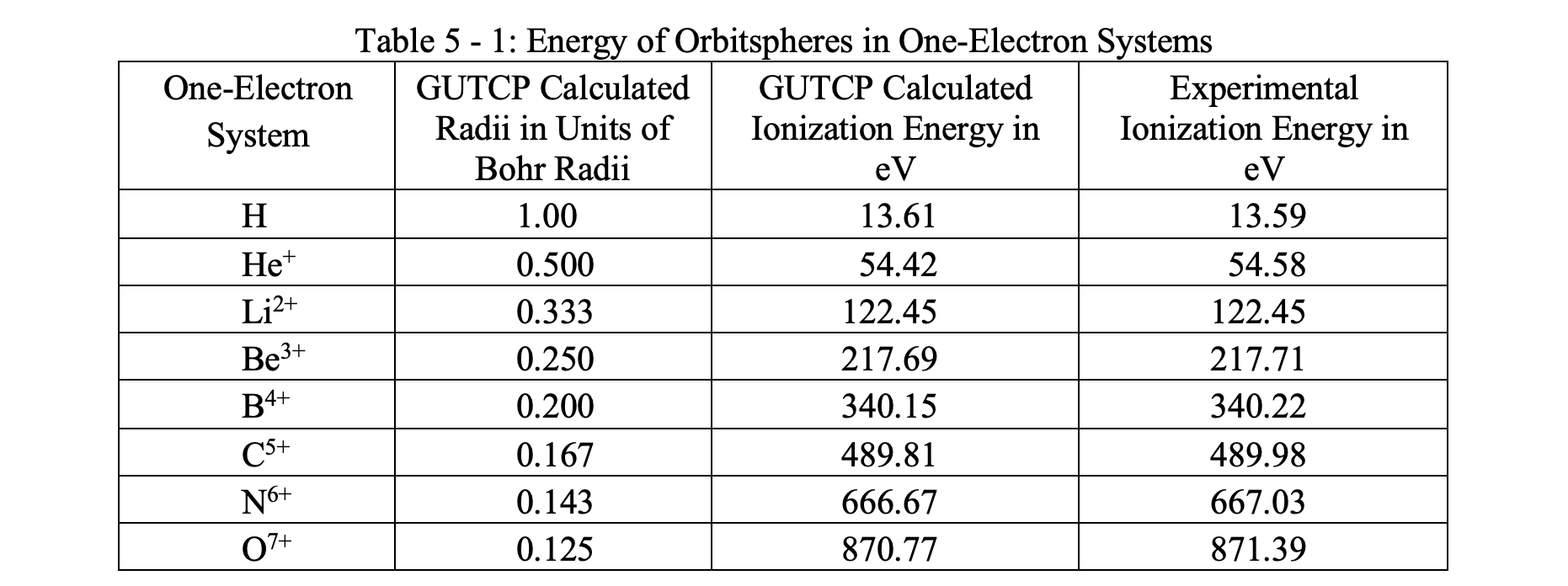
As noted in previous chapters, the tiny deviations of calculated values from experimental values disappear when an additional small relativistic correction term is applied, resulting in theoretical values that match experimental values to within the margin of experimental error.
Example II of OPD: Two-Electron Systems
The spectra of helium and many two-electron ions are known from a multitude of observations made in many laboratories. The basic equations of the force balance for one and two-electrons atoms and ions are the same, but the latter requires an additional force term due to magnetic interactions.
Indeed, the second electron, required to form the complete neutral helium atom, approaches an ionic core in which the net electrostatic attraction is that of one proton, as the fields of the inner electron/orbitsphere symmetrically cancels that of one of the two nuclear protons.
In addition, the force balance is modified, relative to that employed to describe the inner electron, by the magnetic interaction between the two electrons. All of this is described in more detail in the preceding chapter and, as noted, leads to Eq. 4-17, with no variable parameters, of the previous chapter.
The first approximation for the ionization energy of the second electron is seen in Eq. 5-1 below. This equation is in fact a classical physics result of Maxwell’s equations (1872):

This first approximation equation, for ionization energy, clearly does not require a supercomputer to solve, but rather only a very basic calculator or a good head for numbers and an envelope with a clean back. The results of this equation can be employed to predict the first ionization energy of all two-electron systems, simply by changing Z to equal the number of protons in the ion core.
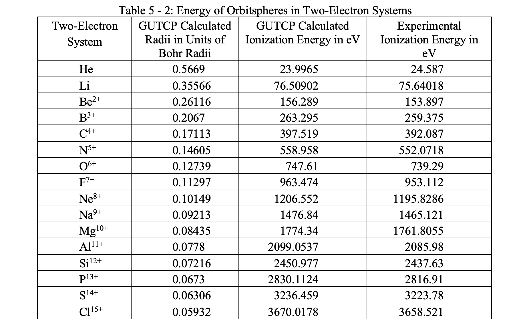
As shown below in Table 5-2, the predictions of the model and the measured ionization energies, for a series of two-electron ions with increasing Z (protons), are astoundingly close to the experimental values.
One energy correction not considered/included herein is “magnetic energy.” The small difference between measured and predicted energy may be attributed to ignoring this small term and a “relativistic” correction term, or possibly experimental uncertainty. The further correction terms included in the Source Text for “magnetic energy” are not related to any of the magnetic force terms discussed herein.
The net impacts of these corrections on the predicted energy of all ionizations are very small, generally far less than 1%. It must be noted that including the corrections in the computation do very marginally improve the agreement with experimental data. However, the theory underlying these small corrections is undeniably very complex, clearly beyond the scope of this monograph. Hence, for reasons of brevity, and to reduce distracting complexity, no discussion of these minor corrections is found herein.
There is nothing remotely similar developed for SQM. For every atom and ion, a new and massive calculation is required to curve fit known data using at least two variable parameters.
There are those who would reject the GUTCP process because it is not in absolute perfect agreement with data. In some cases it is claimed SQM computations get closer to measured values than the GUTCP predictions. But this is not the real disturbance for this community as clearly, measured values always have some element of uncertainty, and the GUTCP predictions are clearly extremely close to measured values, and in the opinion of this author, an experimentalist with 45 years of experience, easily within the margins of experimental error.
The real problem for the mainstream physics community: the notion that the outer electron radius and ionization energy can be determined from a simple algebraic equation in which Z is the only variable, a non-adjustable parameter, is heretical.
They must find some objections.
There are many problems with the “SQM can do better in a few cases” objection. First, the SQM computations are based on “approximations” to the actual SQM theory. And the real SQM theory is fatally flawed to start. It only produces a probability distribution for the whereabouts of an infinitely small electron. It requires 3N dimensions where N is the number of electrons.
Exactly where are the lithium electrons in nine-dimensional space?
SQM ignores Newton’s Laws, has no provision for the known magnetic fields of elementary particles to impact quantized energy levels, is full of incalculable infinities, creates “throw-in” non-theory based concepts like “correlation” to sleight-of-mathematics around infinities, etc. (see Chapter 4). The approximation theories which are actually employed in the computations, assume all systems, all N-values, are in three dimensions. These massive “approximations” (e.g. three dimensions vs. nine) suggest these “approximations” are actually better denoted pseudo-theories. And they are not predictive at all. They are simply curve fit routines.
The merry-go-round of computations for pseudo-SQM theories only stops when the adjustable parameters are finally adjusted such that the difference between the curve fit’s computed values and the experimentally measured values are shown to be at a minimum. This is called “optimization.” This generally requires some supercomputer dedicated to the computation for hours.
It is not at all surprising that a curve fit with adjustable parameters can in a few cases get very, very, close to measured values.
In contrast, it is amazing that the GUTCP, based on three-dimensional space, all known classical forces including magnetic, actual physical particles of three-dimensional shape, with no adjustable parameters, and very simple algebra, no need for a computer at all, based on core classical physics concepts, is in such remarkable predictive agreement with data.
In sum, one must choose:
A CURVE FIT based on an optimization routine (SQM) and a selected “approximate” theory, which can only be solved using world’s largest computers, or;
A PREDICTION (the GUTCP) using classical physics involving simple algebra, no computer needed.
Another common objection to the GUTCP approach is raising the issue of the three-body problem, a class of problems for which no closed form solution exists. However, this objection belies a total lack of understanding of a core principle of the GUTCP orbitsphere model, in which spherical symmetry of electrons reduces the atom to a one-dimensional problem.
You can lead a horse to water, but you cannot make him drink.
EXAMPLE III of OPD: Three-Electron Systems
One-electron and two-electron systems described above are brief reviews of the previous chapter. Next, the discussion moves to a new level of complexity: the GUTCP prediction of the ionization energies of all three-electron atoms and ions using the basic force-balance concepts described above. (Authors accolade: This single chapter of the Source Text is The Greatest Achievement in the History of Atomic Physics. Even perusing this chapter in the Source Text is an utterly stunning experience).
The algebra involved can become quite involved, primarily because of the details of determination of the net magnetic force acting on each electron; hence, only three-electron systems are described in detail. Solutions for systems with up to twenty-five electrons, including descriptions of the derivation of magnetic force terms, are provided in the Source Text.
Li2+, Li+ Li0
Calculating the energy of the innermost electron in Li, the single electron of Li2+, is simple, as it is one of the one-electron systems described in detail in Chapter 4. As shown there, combining the force balance and the conservation of h-bar of angular momentum equation leads to a simple equation for radius:

Once r is determined, the energy is computed using Eq. 5-1. The results for all one-electron atoms, including Li2+ for which case Z=3, is given in Table 5-1.
For Li+, the two-electron/three-proton ion, the program is to employ the same approach as that described in detail for He0 (Chapter 4), which results in an electron structure which corresponds to that of helium. Specifically, in this author’s Mod 1 model, like the two electrons in He0, the two electrons in Li+ do not follow the PEP. Each has a different radius and a different energy.
The Li+ model presented herein is distinctly different than that presented in in the Source Text. In the Source Text, both radius and energy are the same for the two electrons in Li+.
To demonstrate this, the Li+ radius equation is copied in this excerpt from Chapter 10 of the Source Text:

The two electron orbitspheres in the GUTCP model slide/spin by each other, actually superimposed, according to the Source Text.
Given that the two electrons according to the Source Text are co-incident, what is the energy of the electrons? Are the energies also the same (“degenerate”) or nearly so? The energy of the two electrons is also considered degenerate. To quote the Source Text, Ch. 7:

In sum, in the Source Text, kinetic, potential, and total energy are all only a function of the radius of the orbitsphere, hence the two inner electrons of lithium have the same energy.
Returning to the Mod 1 model presented in detail in Chapter 4: a simple equation for radius derived in the Source Text by combining the force balance with the conservation of angular momentum is developed in Ch. 4, (Eq. 4-19) and repeated here for convenience:

This equation is valid for any two-electron system: only the value of Z changes. In Chapter 4, Z=2 for He0 was described in detail. For Li+, this equation is valid with Z set to 3.
The following is a computation of the radius and energy for the outer electron in the Li+ ion.
Re-organize Eq. 5-3 by multiplying through by r3, solving for r, to yield for the Z=3 case:

The result is that er2= 0.355 a0 (Table 5-2), whereas er1 = 0.333a0 (Table 5-1), where erx is the electron at radius rx.
The two electrons have distinct sizes and are not in any manner “co-incident.” To re-state for emphasis: in this monograph we offer, herein for three-electron species, a general modification (Mod 1) of the Source Text regarding the radius and energy of the two inner electrons such that they have neither the same energy nor the same radius. The reason for this is explained in detail in Chapter 4.
Next, we apply Eq. 5-1 to obtain the energy of the two electrons in Li+, noting that the value for Z-1 = 2 is correct, as the outer electron effectively has a central Coulombic force of 2 protons.
Equation 5-1 is initially in Joules, then converted to eV using the conversion factor:
1J = 6.242*1018 eV.
Once again, the two electrons have distinct energies:
Eer1 = -122.45 eV (Table 5-1)
Eer2 = -76.5 eV (Table 5-2)
Where Eerx is the energy of the electron at radius rx.
Clearly, the two electrons in Li+ are not degenerate according to the Mod 1 GUTCP model, in which bound electrons are never degenerate in either radius or energy.
Note: this model is completely consistent with the rejection of the Pauli Exclusion Principle introduced in the last chapter. Indeed, in SQM the two electrons of Li+ have identical energies, wave functions, and in fact are only different in that one electron is spin up and the other is spin down. That is, SQM assumes the PEP.
In this monograph there are never two electrons with the same energy or radius. The PEP is rejected for all atomic species.
It is important to note that in the analysis presented herein, as in Chapter 4, that the outer electron (er2) does not act on the inner electron (er1). Applying the zero orbitsphere interior field model of this monograph, the size and energy of the inner orbitsphere is not impacted by the addition of a second/outer electron.
Why? As discussed in more detail in Ch. 4, Mod 1 model, there is neither an electric nor a magnetic field inside a superconductor, so there is no field generated inside er2 that can modify the forces acting on er1. Hence, the size and energy of er1, even in the presence of er2 and er3, is perfectly predicted by the force balance and angular momentum equations described for Li2+ (Eqs. 4-5 - 4-7).
The Source Text and the Mod 1 models are clearly distinct. Notably, in the Source Text there is a constant magnetic field inside any orbitsphere, not a zero field as postulated in this monograph. This modifies the approach taken and results in different predicted energies for the orbitspheres for the two models.
In the Mod 1 model the energy and radius of the two Li+ electrons are distinct, whereas in the GUTCP model they are degenerate. Only the Mod 1 Exclusion Model avoids the energy conundrum illustrated in Figure 5-1 below and discussed in detail in Ch. 4.
The Lithium Atom
The final step in the development of the lithium model is to add the third and final electron, converting Li+ to Li0.
Same questions: What is the size of the er3 orbitsphere, and what is the energy of the outer electron? And to provide a quantitative answer, the same approach is employed, development of a force balance.
The key difficulty is developing an expression for the magnetic force of the two inner electrons operating on the third electron, er3. Superficially, it appears that there should be no net magnetic force. Indeed, as the spin orientation of er1 is opposite to that of er2, and as the magnitudes of fields each independently creates for r> r2 are identical, by the rules of vector addition they should perfectly cancel for any r>r2.
Moreover, even before solving the force balance for radius and energy, it is clear r3 > r2 by virtue of the reduced Coulombic force on er3. Indeed, er3 only feels the net field of a net single proton, thus to a high-quality first estimate should have a larger radius than er2. In sum, superficially, it appears there is no net magnetic field created by er1 and er2 acting on er3, hence, the force balance on er3 need not have a magnetic term.
Contrary to the above suggestion that the two electrons er1 and er2 have no field for r>r2, a GUTCP postulate of atomic behavior per the Source Text, one also accepted in Mod 1, is that there is a net diamagnetic field created by the two inner electrons. And note, a diamagnetic field is repulsive, not attractive. This field is postulated to have this formulation, a formulation accepted in Mod 1 as well:

Note that this force equation is clearly anchored in three-dimensional reality, has the correct dimensions, and “looks” like standard models of magnetic force. For these reasons it is accepted herein as a reasonable classic physics force equation, and thus is consistent with the requirement of GUTCP that all physics is classical physics, pre-1872 physics, at all scales.
In the Source Text, detailed and complex derivations from classical physics of the magnetic terms in the force balances are developed.
However, for purposes of this manuscript, it is reasonable to simply accept the magnetic terms as postulates.
As discussed elsewhere in this text, physics postulates abound. Indeed, even the most common classical equations, such as the 1/r2 force equations associated with gravitational and electric fields, were not presented by a Supreme Being. Those relationships were postulated by scientists and tested.
A more questionable example of postulated relationships and rules are the innumerable and improbable postulates of SQM. Example of dubious postulates in SQM include:
The required failure of Newtonian mechanics at scales of h-bar and smaller.
The requirement that particles are probability distributions of infinitely small charges rather than 3-dimensional objects with defined shape.
Magnetic behavior of these particles is simply postulated to have a precise magnitude and is not, per classical physics and Special Relativity, associated with current.
For systems of more than one electron (N-electrons), there are 3N dimensions, etc.
In any event, the correct rule of any empirical science, including physics, is: those postulated relationships that provide predictions, particularly quantitative predictions, that accord with observed behavior are accepted.
In this case, the form of the diamagnetic field presented in Eq. 5-5 was tested and found to lead to the measured value of the ionization energy again, and again, and again, as discussed below.
For this reason, the postulated diamagnetic force term is deemed “viable.” Moreover, it appears to be consistent with either the zero-interior field (Mod 1) or the constant interior field (GUTCP) models. In terms of the former, it is argued that the field of er1, not zero for r>r1, is not fully cancelled by the electron at radius r2, such that the net magnetic field beyond er2 is non-zero.
No attempt to quantify is provided herein. An argument for a non-zero magnetic field for the GUTCP constant interior field model for r>r2, and its magnitude, is provided in the Source Text.
In any event, both models, GUTCP Source Text and GUTCP Mod 1, yield the same force balance for the outermost electron, er3, in Li0:

Given that the equation for r2, and noting s=1/2, the equation the earlier developed for r2, (Eq. 5-4), Eq. 5-6 becomes:

Which yields r3 = 2.5559 a0.
The equation for the electrical energy for the outermost electron is consistent:

Given the value of r3 computed using Eq. 5-7, the ionization energy of the outermost electron in Li0 is 5.32 eV, a value within 2% of the “experimental’ value of 5.391 eV.
Note: there is reason to question the number of digits of accuracy the experimental value can reasonably claim; hence, it can reasonably be argued the GUTCP predicted value is in excellent agreement with the range of reported observed values.
Additionally, further small corrections in the Source Text yield energy values generally closer to the accepted experimental values than those reported herein. These small corrections are not, as discussed previously, included in this monograph for reasons of simplicity.
Indeed, the derivation provided in the source text is too complex to allow a compelling explanation to be provided herein in a reasonable fashion. In any event, a difference between predicted and measured values no larger than 2% based on the first principles argument provided above, and the uncertainty of the measured value, is a spectacular achievement.

Figure 5-1: Energy Levels of Li Mod 1 vs. GUTCP vs. Measured. As shown the Mod 1 quantized energy level values match the measured energy levels. In addition to not matching the measured values, the GUTCP model for Li+ involves an energy conundrum. From the right panel “GUTCP” these questions arise: i) Where does the energy go when one electron initially at -75.6 eV (GUTCP model) drops to -122.4 eV during the ionization process? Note the ? mark on the “relaxation” process, right side. ii) Once double ionized, from what source is energy provided during electron capture (Li2+ -> Li+) in order for the electron at -122.4 eV to return to the GUTCP predicted energy of -75.6 eV? These questions do not arise for the Mod 1 Model; hence Model 1 has no energy conundrum. See Chapter 4 for a more detailed discussion of this conundrum.
Summary of Difference for Li0 for GUTCP vs. Mod 1
As noted above, there is a departure from the approach used in the Source Text in this monograph. In the Source Text, the inner two electron orbitspheres (er1 and er2) are considered to be co-incident. Both have the same radius, and that is the radius of the inner electron. The two electrons also have the same energy.
In contrast, in the Mod 1 model the two electrons in Li+ have very distinct radii, and there is no Pauli Exclusion Principle. Second, in this manuscript the two electrons of Li+ are not degenerate. The same energy conservation logic described in Ch. 4 for He0 must apply here as well. Indeed, it is experimentally thoroughly established that the first and second ionization energies for Li+ are very different. As listed in Table 5-2 the first ionization energy is 75.6 eV and the second (ionization of Li2+) is found in Table 5-1, 122.4 eV.
This is an energy conservation conundrum.
Below, an abbreviated argument for the nature of the energy conundrum is provided. (It is abbreviated because it follows precisely the same logic as that developed for rejecting the Pauli Exclusion Principle developed in Chapter 4 for helium. The reader is urged to review the full argument, fully illustrated, there.)
Assume the PEP is correct. If the first electron in Li+ is removed with a 75.6 eV photon, the second “falls” to 122.4 eV, as it must to be consistent with the well documented/measured ionization energy for Li2+. This appears to be the GUTCP energy level model, as discussed above (Figure 5-1).
This model immediately raises a couple of energy conservation question: where did the difference in energy between initial and final states for this un-ionized electron, ~47 eV, go as the un-ionized electron fell in energy to its final state? And once Li2+ recaptures an electron, and once again becomes Li+, with a known energy release of 75.6 eV, where does the required energy ~47 eV, come from to increase the energy of the electron, initially at -122.4 eV in Li2+, back to its Source Text postulated energy for Li+ of -75.6 eV?
In actual experimental fact, electron capture by Li2+ releases 75.6 eV, consistent with the energy change between a free electron and a Li+ outer bound electron.
As shown in Chapter 4, the PEP, applied to any atomic system including He and Li, leads to the inevitable creation of energy by cycling between ionized and un-ionized states. That is, the world could be supplied with infinite energy just by cycling lithium between Li + and Li2+ states if the PEP is correct.
Clearly, the PEP is not correct. There is no PEP (Figure 5-1, Mod 1 model).
In sum, Li+, like He, consists of two electrons with distinct radii and distinct energies, one orbitsphere inside the other, like a set of Russian dolls.
Three Electron Atoms, Z>3
The final category of species for which a fairly complete model will be provided in this monograph are ions containing three electrons but more than three protons, such as Be+, B2+, C3+, etc. Once again, determining the ionization energy of these species requires a postulated magnetic term(s) in the force balance, with the Coulombic interaction described as per all earlier described force balances.
The key GUTCP postulate is that the two inner electrons are fully described by the force balances provided in the preceding section for er1 and er2, with appropriate change in Z, but the force balance on er3 is significantly modified. Specifically, given the fact that there are insufficient electrons for Z>3 to cancel the field from the nuclear charges beyond r3, there is positive electric field that interacts with the B-field of er3. Contrast this with lithium. Beyond the outermost electron of lithium, in all models there is no net magnetic field.
In sum, the GUTCP takes account of the fact that in classical physics any ion, such as Be+, with more than three protons, but only three electrons, will have an electric field/ion field beyond its outermost electron. This leads to the inclusion of a new force term in the force balance.
Moreover, a precise formulation of the resulting diamagnetic force can be derived from classical electrodynamics. In the final analysis, this results in three terms in the force balance. The first two are unchanged from Eq. 5-6, but the third term represents a second diamagnetic force for ions arising from the interaction of B and E fields beyond the outermost electron at r3.
In a detailed analysis provided in the Source Text, a diamagnetic force term, derived from classical physics for a charge moving in a central field having an imposed magnetic field perpendicular to the plane of motion. This second diamagnetic force, for the outer electron er3, is postulated to be precisely quantifiable employing this relation:

The total force balance on the outer electron in these ions is expressed as:

In the Source Text, a quadratic in the unknown quantity r3 is derived. Once the quadratic is solved, an expression for r3 is obtained:
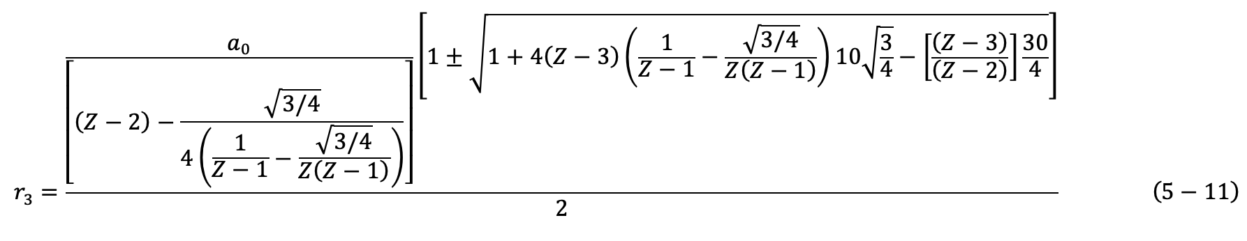
The positive root is the only acceptable real solution.
Note the equation for radius (Eq. 5-11), and the equation for energy (Eq. 5-8) of the third (outer) electron are a simple function of the number of protons.
To determine the predicted radius or energy of the electrons in any three-electron ion, it is only necessary to recompute with the correct Z value in the simple algebraic expressions. Empirically correct for all atoms.
This is remarkable. There is nothing remotely similar to be derived for SQM.
The only unimpeachable data regarding atoms is either the ionization energy based on voltage at which current increases due to ionization of gas phase species, or spectroscopic data which identifies the energy of the reverse process, electron capture. Both provide quantized energy levels for atoms.
For this reason, the energy values, specifically ionization energies, available for atoms and ions from reliable sources (e.g. NIST) are the only reliable means to test the theory. Indeed, if the GUTCP predicted energy values match the measured values, then the theory retains its validity. Physics is empirical.
The predicted and measured values match extremely well. In Table 5-3 the predicted values of electrical/ionization energy for three-electron species, atoms and ions (Eq. 5-8) are compared to measured values.
Notably, in the Source Text (Table 10.1) the predicted ionization energy values are corrected for magnetic energy of ionization and relativistic effects. This leads to even closer match between measured and predicted values; however, as noted above, those corrections are not included herein for several reasons. And yet, the match without any correction and no variable parameters, is still remarkable!
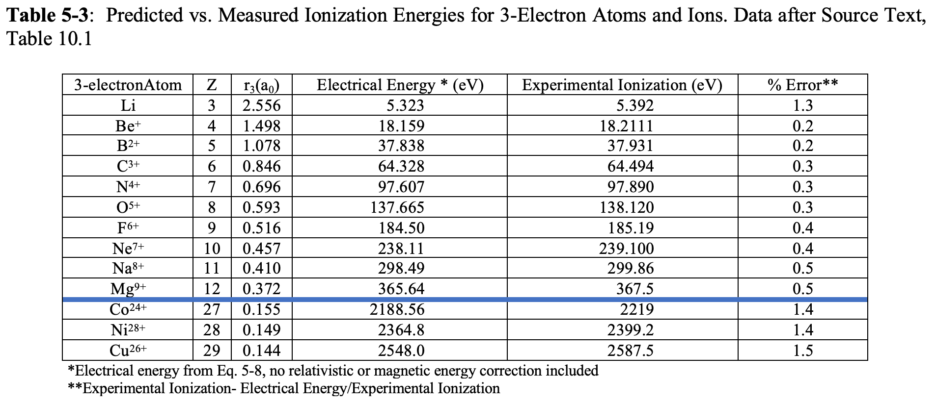
Computations for all three-electron atom values Z=3 through Z=29 are available in the Source Text, Table 10.1.
A few other remarks regarding this model of three-electron ions are in order. First, is this second diamagnetic term in the force balance significant? A few “test” computations, based on this computed ratio:

And the values given in Table 5-3 reveal that the second diamagnetic force term is larger than the first, of the order 1.5 times larger. In sum, it is significant.
Second, are the magnetic corrections to the force balance significant? To answer this question, a ratio of Fdiamag1 to the Coulombic force term is evaluated:

Using C3+ as an arbitrary example, and the computed r1-value (0.171 a0), the ratio of forces computed form Eq. 5-12 is approximately 0.32. Given that the second diamagnetic force is generally larger, the computed ratio leads to the general conclusion that the Coulombic and magnetic forces acting on the electrons in atoms and ions are generally of the same order of magnitude. Thus, both the magnetic and the Coulombic terms are required for accurate computation.
EXAMPLE IV: GUTCP Predictions Vs. Data For Larger Atoms
The same approach outlined above for atoms with three electrons (Z=3) and ions with Z>3 is employed for atoms for systems with four or more electrons. The same approach is employed:
Develop a force balance including the Coulombic force and all magnetic forces.
Rid the equation of the velocity term using the fact that the angular momentum (mvr) is always h-bar.
Solve the resulting single variable (rx) equation for the radius in question.
Substitute proper r and Z values into energy equations, generally Eele although in the Source Text there is often small correction for magnetic energy associated with the ionization process. The comparison between GUTCP and data for systems of four or more electrons confirms GUTCP is a validated theory for all atomic scale systems.
Note: in general, the most difficult aspect is development of the magnetic force terms.
Once again, it is found that an equation developed for a particular ion will have a variable Z, which is modified to obtain the correct radius and ionization energy of all ions with the same number of electrons.
It is found there is a remarkable and irrefutable agreement between accepted observations and the GUTCP predictions.
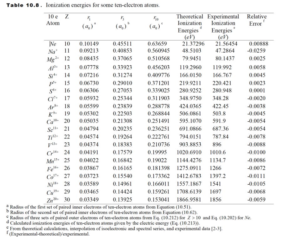
An example of the outcome of this relatively simple (i.e. compared to SQM) process, specifically for ions with ten electrons, is provided in Table 10-8 seen below, excerpted from the Source Text.
Once again, the classical physics-based approach with simple force balances and absolutely no variable parameters, shows extraordinary agreement with data. As pointed out in the text, the magnitude of the difference in energy between the computed values and the measured values are well within the error range of the imperfectly measured values.
Critics who deride this as “numerology” or worse clearly have not studied the GUTCP and do not understand the scientific process.
Iron Ions
In response to the young lady from Chapter 1 who inquired regarding the application of quantum mechanics to transition metals, the data provided below shows: the GUTCP predictions match the observed spectroscopy of transition metal atoms.
And as her professor noted: the current accepted paradigm, SQM, cannot even predict the spectra of helium. SQM is only a curve fitting routine beyond hydrogen!
Another question: how simple is GUTCP? Can this model be used to predict quickly, no computer needed, the ionization energy of an atom in all of its ionization states? The answer is yes.
As iron ions are considered to be the source of some odd radiation in intergalactic clouds by the mainstream scientific community (discussed in Ch. 9), this author decided to build a table of values of ionization energy for a set of Fe ions from the tables for many electron atoms.

In conclusion, the GUTCP atomic model success indicates it has supplanted SQM as THE Quantum Theory for atoms and ions. The fact that the GUTCP allows precise predictive model of the energy levels in atom and ions using only simple classical physics and no variable parameters, already makes it one of the Great Theories of Physics, in a class with Newton’s Laws, Maxwell’s Equations and Relativity. And by extension this achievement alone means Dr. Mills is one of the towering figures in the history of physics.
Personal Note
Once persuaded that the GUTCP is the only viable atomic theory, I was freed to reconsider all of physics. In college there were topics for which the physics I was taught seemed inadequate, but I didn’t feel entitled to question wisdom developed by great thinkers over centuries. Just accept. And my attitude was the same as virtually all physics students and working physicists! This is still the dominant thinking. Only a few have escaped the “experts rule” trap in the interim.
My reasoning changed due to the success of the GUTCP. If the GUTCP, developed by a true physics outsider, provides a far superior explanation of atomic spectra than SQM, perhaps even I was entitled to challenge aspects of the standard physics model.
In other words, the GUTCP gave me courage and inspired me to think outside the standard paradigm box. Perhaps this essay will inspire others to have courage and then challenge the standard paradigm. Incidentally, Randy is way ahead of me. The Source Text is a spectacular, near infinite, reconsideration of almost all of physics.
The first question I raised, once emboldened by the GUTCP: what are the kinetics of electric and magnetic field formation and dissolution?
This question puzzled me in college. To understand my puzzlement, it is only necessary to consider this issue using a simple physical example.
To wit: experimentally, there is no electric field from a hydrogen atom, but experimentally it is clear upon ionization two fields are detected, one from the electron, one from the proton. How long does it take for these fields to form after ionization? Do they grow in time?
And conversely: after the proton recaptures the lost electron to reform the original hydrogen atom, how long does it take the two fields to disappear? Do they gradually shrink?
Remarkably, these questions are not even addressed in the physics literature (nor in the Source Text)! Is the answer so obvious it can be ignored? Not to me! Thus, considering these questions was an opportunity for me to do my own (original) thinking!
The answer I conceived can be called the everything is everywhere all the time model.
The fields of charged elementary particles are a permanent component of the particle. These fields are the size of the universe and never change. Energy is never taken from or given to these fields, except in the form of photons, which in this model are waves on an infinite field, which are analogous to seismic waves in the earth. Indeed, like seismic waves, the photons of the universe do not interact directly with each other.
Atomic hydrogen has no apparent field because of yin-yang: outside the GUTCP atom, the positive field of the proton is exactly cancelled by the negative field of the electron due to spherical shape of the electron. Spherical symmetry leads to perfect apparent cancellation.
Both fields are simultaneously present at every point in space, but because they precisely cancel, it is impossible to detect them. For example, the net effect of the electron and proton of a hydrogen atoms on any other charged particle is zero. The field of one (e.g. -) pulls on the charged particle with energy Y in one direction, and the field of the other (e.g. +) pushes with the same force in the opposite direction. The net force is zero. (Note: magnetism is a “not cancelled” component of fields of net neutral material, more below.)
Thus, the answers to my questions are that the fields don’t grow and shrink, they simply become “visible” once the spherical symmetry of the atom is broken. Ionization breaks that symmetry. There is no longer an electron orbitsphere surrounding the nucleus, resulting in net field cancellation. Instead, there are two physically separated charged particles that create a net dipole field.
The process of electron capture/hydrogen atom reformation, re-establishes the symmetry, leading to net field cancellation. The dipole appears to disappear.
In this new model, every charged particle is no longer to be considered a very small, even infinitely small (SQM), but rather an enormous particle, possibly the size of the universe. Every charged particle consists of a very small solid component, per the GUTCP, and a field component the size of the universe if that particle was born at the Big Bang, the current standard paradigm for the initiation of the universe. (Notably, Randy is not an advocate of the Big Bang model.) The model requires that the fields do not interact with other fields, but only with the mass components of other charged particles.
Is the model consistent with all known phenomena? I argued YES in my published, but never read, introduction of this theory:1
J. Phillips, “Required field structure of extended three dimensional charged particles,” Physics Essays 23(4), 574–578 (2010).
For example, it is easily shown to be consistent with all aspects of Special Relativity. Indeed, the two requirements of Special Relativity are:
The equivalence of all inertial reference frames.
The speed of light is constant in all reference frames.
Assume each electron is an inertial reference frame. As required, all electrons are identical and the speed of light in the field of each electron (remember each has a field the size of the universe) is the speed of light.
Next, Special Relativity explains magnetism. Does this model also explain magnetism? According to Special Relativity magnetism as simply an expression of the electric field acting perpendicular to the vector joining two charged particles moving relative to each other. In other words, there is no magnetic field apart from the electric field.
If there is no magnetic field in the absence of an electric field, per Special Relativity, a question arises: how can a chunk of iron, which clearly has no measurable electric field, have a magnetic field extending over all space? Isn’t this contrary to the theory of Special Relativity?
The answer from my model is that the chunk of iron does have an electric field everywhere!
The “electric” part of the iron field is net zero as the field from the iron atoms’ positive charges cancels the charges from the equal number of negative charges at any point in space. However, the relative motion of the negative charges (orbitspheres) is not matched by motion of the nearly non-moving positive charges. The negative charge is whirling around in great circle current loops, and the positive charge is also spinning but producing a far smaller magnetic field (mag moment of an electron/mag moment of a proton ~700) than that of the electrons.
Net result: the “magnetic” component of the iron, arising from the motion of negative charges relative to the reference frame of the iron chunk, is not cancelled by a counter motion of positive charges relative to this same reference frame. Hence, a net magnetic force is felt by charged particles near the iron. And on and on… The interested reader is referred to the published paper.
A couple of additional comments are germane here.
First, Randy contributed, inadvertently, to my thinking on this subject. Decades ago, he explained to me in his office that one of the inspirations for the GUTCP model of the orbitsphere was the lack of any evidence of a dipole field of an atom. He concluded the electron CANNOT be a moving zero-dimensional particle as that would inevitably create a dipole of some kind. This led to the notion that the bound electron must be spherically symmetric relative to the nuclear particle.
That remark caused me to add a new criterion to my model building: models must be both self-consistent and consistent with ALL observations. One cannot leave out inconvenient observations.
In the case of fields, a viable model CANNOT require fields to blink in and out of existence. That is not self-consistent with the notion that fields have energy. Where does the energy go upon “blink-out” and where does it come from on “blink-in?” It is also inconsistent with the failure to observe fields growing or shrinking in time.
In contrast, the model that I propose, in which the field of every particle is forever and everywhere, is self-consistent and, surprisingly, consistent with all observation. Particle fields only gain or lose energy via a photon mechanism.
Second, I did try to publish this concept in several major journals. They all refused to even have it reviewed. Only Physics Essays sent it for review, then accepted it after very positive reviews. One might reasonably conclude the major scientific institutions are not interested in paradigm shifts.
Surprise!
I have a very good citation record, a dozen papers with more than 100 citations (Google Scholar), and more than 6600 total citations. (Very good? Compare: my old college roommate has a great citation record with more than a dozen papers with 1000+ citations). Unfortunately, my best papers, like the one cited, are absolutely ignored!
Has anyone in the prestige physics community found the close match with experimental ionization values by these classically-derived formulas remarkable? The close match with experimental values by formulae derived from classical physics can't have gone entirely unnoticed by the entire SQM community. They already accept, as reasonable computational approximations, the single electron Bohr model calculation of ionization energies. At the very least, these formulas could be tacked on to the Bohr model with no less legitimacy, if for no other reason than that they provide approximations of relatively impractical QED calculations.
I agree with your comment. I only hope that Dr Mills see it and responds with an explanation.