


The Hydrino Hypothesis Chapter 7
An Introduction To The Grand Unified Theory Of Classical Physics

This monograph is an introduction to Randell L. Mills’ Grand Unified Theory of Classical Physics, Hydrino science, and the efforts of the company Brilliant Light Power (BLP) to commercialize Hydrino-based power technology, as told by Professor Jonathan Phillips. Out of necessity, it assumes a degree of familiarity with physics and physics history. An overview of the BLP story which serves as a helpful introductory piece to those unfamiliar with its sweeping scope can be found here. Readers should also read the previous chapters of this monograph prior to this one:
Chapter 1 of The Hydrino Hypothesis
Chapter 2 of The Hydrino Hypothesis
Chapter 3 of The Hydrino Hypothesis
Chapter 4 of The Hydrino Hypothesis
Chapter 5 of The Hydrino Hypothesis
Chapter 6 of The Hydrino Hypothesis
By Professor Jonathan Phillips
The Hydrino Hypothesis
Preface: This chapter marks a break in the narrative. The prior chapters focused on the theories of the GUTCP and SQM, and the quantitative match between the predictions of the GUTCP and data gathered over more than 100 years regarding accepted forms of matter. In particular, the prior chapters focused on the GUTCP predictions, compared to the curve fitting of SQM, to spectroscopically determined energy levels of electrons in atoms, ions, and excited states.
The following chapters are focused on forms of matter predicted to exist by the GUTCP, forms that current theory deems impossible.
The GUTCP proposition, one that is not only rejected but actively disparaged by most in the scientific community, is as follows: the electron in hydrogen atoms can literally shrink, forming a hydrogen atom orbitsphere smaller than the standard ground state orbitsphere (n=1). These smaller hydrogen atoms are called Hydrinos.
One aspect of the Hydrino Hypothesis (HH) is that creation of Hydrinos from hydrogen atoms leads to the release of tremendous energy. It is estimated that on average converting one hydrogen atom to a Hydrino state releases 200 times more energy than burning one hydrogen atom to generate water. BLP is working on technology to create Hydrinos and convert the energy released from their formation into electrical energy. Creating Hydrinos is envisioned as an inexpensive new primary form of clean energy, with the potential to transform the energy landscape for civilization.
The first chapter in this section outlines key points of the Hydrino Hypothesis, and lists observables predicted to exist by the theory. Subsequent chapters in this section are focused on the excellent quantitative match found between prediction regarding Hydrino formation and observation. These chapters include a review of the literature showing there is no data that debunks the Hydrino Hypothesis; hence, the Hydrino Hypothesis remains valid.
Introduction: The Hydrino Hypothesis
GUTCP predicts there exists a process for creating bound hydrogen electron orbitspheres that are stable, physically smaller, and lower in potential energy than deemed possible in standard physics. A more conventional manner of expressing this: the GUTCP predicts that there are energy states of the electron in a hydrogen atom that are stable and lower in energy than the standard “ground state” for hydrogen. Dr. Mills has dubbed these states “Hydrino” states of hydrogen.
The GUTCP predicts that tremendous energy is released during the formation of Hydrino states. If this energy can be captured and harnessed, it can provide an amazing new primary energy source. The efforts of Brilliant Light Power to engineer a Hydrino-based power device are discussed in this overview article.
Hydrino Formation Conditions
The Hydrino formation process is postulated to take place in two steps under specific conditions. The required conditions are as follows:
The presence of atomic hydrogen. Hydrogen is extremely common on earth in molecular form, most often as part of the water molecule (H2O); however, pure hydrogen molecules (H2) are very rare at pressures and temperatures normally found on earth. Far rarer is atomic hydrogen (H), a chemical radical, reacting with virtually any other species quickly, thus only present under certain extreme conditions, such as in plasma discharges.
A Hydrino catalyst species. In the GUTCP Source Text Hydrino catalysts are certain atoms, ions, or molecules that can accept a specific amount of energy from atomic hydrogen: an integer multiple of 27.2 electron volts (aka one Hartree).
Step 1 of Hydrino Formation
The GUTCP postulates that if atomic hydrogen transfers energy to a catalyst species via a catalytic, non-radiative process called resonant transfer (RT), which requires physical proximity (i.e. collision or field coupling), the electron in the traditional atomic hydrogen ground state can drop to energy levels below the “ground state.” These Hydrino states are physically smaller than ordinary ground state hydrogen.
In the first step of the process, atomic hydrogen transfers m*27.2 eV to a catalyst species that can accept that amount of energy. This energy transfer leads to the formation of a Hydrino transition state, which exists at the same radius as ground state hydrogen, the Bohr radius. However, the transition state is not in force balance.
The energy transfer process may, depending on the type of catalyst, result in either the catalyst ionizing or gaining very high kinetic energy. As discussed below, there are three main categories of Hydrino catalyst species.

Figure 7-1: Type I Catalysts- Atomic catalysts capable of accepting m*27.2 eV (m is any natural number less than 137) receive that amount via resonant transfer, with the atomic hydrogen electron falling into an allowed “transition state” at -m*27.2 eV after the energy transfer to the catalyst. The transition state hydrogen then falls into one of 136 Hydrino states in a second step. Energy is conserved. This process ionizes the catalyst as shown, top right. Upon recapture (later!) of the electron ionized electron, a photon with energy of m*27.2 eV is released. This photon can generate useful energy via photovoltaic capture or simply by rapid conversion of electromagnetic energy into heat. Energy is also released as transition state hydrogen falls into a Hydrino state in the form of high-energy continuum radiation or third body energy.
To summarize Step I of the Hydrino formation process:
Hydrino transition state creation is initiated with a very specific collision: a ground state hydrogen atom collides or undergoes field coupling with a catalytic species that can accept m*27.2 eV.
The transition state forms via a non-photon mediated energy transfer process (RT) between the electron in the hydrogen atom and the catalyst. The RT process, per GUTCP, creates a trapped photon in the transition state that effectively increases the electron-proton interaction strength.
The Hydrino transition state exists at the same radius as “ground state” hydrogen, but out of force balance due to the presence of this trapped photon and its effect on the central field experienced by the transition state’s electron.
Comment: is point 1 above a non-standard assumption? No. In fact, it is generally presumed that most chemical processes require collision between species and generally take place without radiation. Collisions leading to the reaction of two species, atoms, and/or molecules to form net lower electron energy species occurs without the release of radiative energy. These processes are ubiquitous in nature and wholly non-controversial. For example, molecular hydrogen is formed when hydrogen species collide.
In the Source Text many examples of processes in ordinary chemistry occurring without photon involvement are given. One example:

Comments And Questions On Step I
Energy Transfer
The energy transfer from atomic hydrogen to the catalyst species must equal almost exactly m*27.2 eV, where m is any natural number <137. How close must the absorbed energy be to m*27.2 eV? The answer is not clear to this author, and the Source Text does not offer an explanation. This will be an area for future study.
Energy Holes
Dr. Mills has coined the term “energy hole” to describe the process of atomic hydrogen transferring energy to a catalyst species. Energy holes are created when a catalyst species is elevated in energy by E = m*27.2 eV by accepting energy from atomic hydrogen. The hydrogen atom is said to have “absorbed an energy hole” in the parlance of the GUTCP.
After absorption of the energy hole, the hydrogen atom’s electron in the ground state moves to a transition state energy of E = -m*27.2 eV below the standard ground state energy where n is any natural number <137. Only at these very specific energy levels is the natural structure of the hydrogen atom capable of hosting the electron in a transition state.
Below, the description of the Step 1 process as found in the 2023 edition of the Source Text is quoted in part:

Comment: In the current standard physics and chemistry of hydrogen, the lowest energy state is at -13.6 eV. Clearly the current paradigm rejects the notions of “energy holes” and “transition states.” In current chemical and physics models of hydrogen atoms there simply are no hydrogen atom electron states of any kind below -13.6 eV.
Energy Conservation In Hydrino Formation
Energy conservation is maintained. For the atomic hydrogen atom’s electron to fall in energy to a transition state the catalyst must increase in energy by the same amount.
Comment: the energy added to the catalyst species is “de-stabilizing,” as it leaves the catalyst in a non-equilibrium state, e.g. ionized (Type I catalysts, discussed below). The “non-equilibrium” of the catalysts will decay back to a stable, equilibrium, state and in so doing produce a “signal” that is observable (Fig. 1). The nature of the signals is predicted by the GUTCP model and is different for different catalyst types (more below).
Transition State Radius And Force Balance
All Hydrino transition states, 136 in all, have the same radius, the classic Bohr radius. However, the hydrogen transition state energy levels are not solutions to a force balance, hence are not stable. This leads to the second step in stable Hydrino formation, discussed below.
According to the GUTCP model, transition states are characterized by a “trapped photon” that forms upon transfer of m*27.2 eV to the catalyst species. These trapped photons superimpose with the central field of the proton and increase the total central force experienced by the electron by m, with the total force being m+1. For example, a hydrogen atom that has transferred 3*27.2 eV to a catalyst would experience an effective central field 4 (3+1) times that of ordinary ground state hydrogen. This increased central force of the trapped photon leaves the transition state out of force balance and is responsible for Step 2 of the Hydrino formation process.
Hydrino Formation Step 2
The second step of the stable Hydrino formation occurs when the electron of atomic hydrogen in the transition state falls to a lower energy level which is a solution to a force balance. This process, which takes place in a tiny fraction of a second after the transition state is formed, releases energy in the form of continuum radiation or third-body kinetic energy. Notably, the energy levels of Hydrinos are all continuation of the Rydberg series to “fractional” state energy values.
Below is a description of a hydrogen atom in the transition state formed by transferring 2*27.2 eV to a catalyst collapsing to the H(1/3) Hydrino state from the Source Text, 2023 edition:

The second step of Hydrino formation, which results in a stable Hydrino end state, is enabled by completion of the first step. Specifically, when the hydrogen electron absorbs an energy hole equal to m*27.2 eV, this leaves the hydrogen electron in an unstable transition state, which quickly decays, releasing energy. How quickly? Small fraction of a second.
Comment 1: Transitional states are unstable, as noted above, because they are not solutions to a force balance.
Comment 2: An imperfect analogy: a ball falling down stairs. At every step/tread the ball is temporarily at a specific energy level (analogous to transition state); however, the position of the ball on any finite step is not a solution to the energy and momentum balances, hence the ball continues downward, perhaps temporarily inhabiting other treads, until it achieves a stable state of energy and momentum at the bottom (analogous to Hydrino state).
The hydrogen atom’s electron releases continuum radiation or third-body kinetic energy as it decays from the transition state to the stable Hydrino state. The electron accelerates radially inwards from one size, the “ground state” Bohr radius, to the final stable Hydrino size. In the case of continuum radiation release, it is analogous to Bremsstrahlung radiation, in which de-accelerating electrons, slammed into a wall in an accelerator for example, release radiation which spans a broad range of k-space.
According to the GUTCP, in the transition state and final stable Hydrino state there is a trapped photon. This is described in the Source Text, 2023 edition:

Comment: As discussed in the Author’s Concerns section (below) there are some puzzles associated with the trapped photon concept in the transition and stable Hydrino states. At the end of this chapter, an alternative model of the Hydrino state and the mechanism to form one is proposed. In this model, Mod II, there is no photon in either the transition or Hydrino state.
Summing For The Two Steps
The first postulate is that there are a set of natural energies within hydrogen atoms consistent with the formation of Hydrinos. The energy of these levels are m*27.2 eV (m*Hartree energy) below the traditional ground state (-13.6 eV) of atomic hydrogen, where m is a natural number <136. Thus, transition states are found at -13.6 eV + -27.2 eV = -40.8 eV, -13.6 eV+ -54.4 eV = -68 eV, etc below the vacuum energy level.
The atomic hydrogen electron can occupy these energy levels, so-called transition states, by absorbing an energy hole provided by a Hydrino catalyst species of precisely the same energy. For example, atoms that ionize with exactly m*27.2 eV can act as catalysts that generate an energy hole. Energy is conserved. As energy transfer from atomic hydrogen to the catalyst occurs, the catalyst’s energy increases by the exact amount of energy the hydrogen atom’s electron energy decreases. Notably, a “trapped photon” is formed during the energy hole absorption.
The state of the electron/trapped photon in a hydrogen atom after absorbing the energy hole is “transitional” as the process does not leave the electron at an energy level allowed by a force balance. Thus, in a second step, an electron in a transition state will quickly fall to a yet lower energy, one consistent with a force balance solution. The energy lost by the electron falling to a lower level is given off as Bremsstrahlung-type continuum radiation or third body kinetic energy.
Once in one of the 136 states allowed lower energy states, the Hydrino is stable, as it is at a level consistent with a classical force balance, albeit modified by the presence of a trapped photon.
Certain spectroscopic signals are predicted by the model for both steps. A scientific test of the Hydrino hypothesis is to look for these predicted signals. Failure to observe them would debunk the hypothesis.
Hydrino Hypothesis Predictions
The Hydrino Hypothesis predicts that Hydrino formation will only occur under specific conditions with specific catalysts. It further predicts the precise energy (and radius) of each of the short-lived transitional states and the final stable states. Hence, the energy of each transition, and the predicted spectra from the transitions, are exact.
This precision permits cold, hard, and objective quantitative testing. There is no “curve fit” provision, and no back-door excuses. The predicted Hydrino formation either occurs or it doesn’t. The predicted energy release is detected, either spectroscopically or via other means, or the Hydrino Hypothesis dies.
In sum, the Hydrino Hypothesis is clearly the most scientifically radical component of GUTCP, yet is easily tested, as required for true scientific theories. Thus, the Hydrino Hypothesis is not metaphysics.
Only objective testing, not partisan polemics, can determine the validity of a model. As discussed in great detail earlier, for a theory to be labelled viable, or alternatively “debunked,” all that is required is testing and comparison of observations with predictions.
If the Hydrino states predicted by the GUTCP do not exist, then the predicted spectra and other predicted signatures will not be observed, and the theory will be debunked. If the predicted lines are present in the spectra under conditions anticipated to allow for transitions to the lower energy Hydrino states, then the theory remains viable.
What is the status of experimental work attempting to verify the Hydrino hypothesis?
To date, after a multitude of tests, and the collection of an enormous amount of data by geographically dispersed scientists with a range of personal positions on SQM vs. the GUTCP, the status is as follows:
No data inconsistent with the predictions of the formation of Hydrinos has been produced.
Some, but by no means all, of this pertinent experimental work is reviewed in detail in the following chapters. And to repeat the primary conclusion:
All data are consistent with the GUTCP theory for Hydrino formation; hence the theory remains viable, attacks from “experts” notwithstanding.
These Hydrino states, per the GUTCP, have smaller electron orbitspheres that are lower energy than the orbitsphere (Bohr radius) of a hydrogen atom in the traditional “ground state.” Just as with the standard state hydrogen orbitspheres, there is no SQM wave/particle uncertainty to these Hydrinos. They have precise size and precise surface current structure.
As discussed above, it must be noted that the theory does not predict the existence of one size of Hydrino, but rather 136 (Figure 7-2). A hydrogen orbitsphere/atom can pass through each size. With each step the Hydrino literally becomes smaller, and with each step, the potential energy (always negative for bound electrons) is reduced, and the energy difference, sometimes very large, between initial and final Hydrino state released as kinetic energy or continuum radiation.
In sum, one aspect of the Hydrino Hypothesis regards the final stable states: hydrogen electron orbitspheres, smaller and lower in energy than the orbitsphere of hydrogen in the standard minimum energy/ground state hydrogen model. The radii of these 136 progressively smaller sized Hydrinos are all less than the Bohr Radius; the size of a hydrogen atom in the standard concept of ground/minimum energy state.
Finally, the theory predicts the existence of very specific spectroscopic signatures associated with Hydrino formation, and thus can be tested in a variety of ways.

Figure 7-2: Hydrino states of hydrogen. The precise sizes and energies of 136 stable orbitspheres which are smaller and lower in energy than Bohr-radius orbitspheres (the traditional “ground state”) are predicted by the GUTCP theory. Mechanisms for the creation of these states are also identified in the GUTCP. These lower energy state forms of hydrogen are called Hydrino/small hydrogen states and are the possible identity of dark matter. (Excerpted from Source Text).
Hydrino Implications
The predicted existence of Hydrinos has many implications. First, it suggests a physical, baryonic (meaning composed of ordinary matter) basis for dark matter: Hydrino states are predicted to have all the properties of dark matter. It is normal baryonic matter, hence has mass and gravity, a known property of dark matter, but the electron in any Hydrino is so deep in an energy well that it takes tremendous energy to boost it up to the next higher stable energy level.
For example, the highest energy stable Hydrino state, H(1/2), has a binding energy of -54.4 eV. Only extreme ultraviolet (EUV) or shorter wavelength radiation is sufficient to ionize this species, hence in standard astronomical practice (only a handful of space-based instruments are capable of detecting EUV light), which only observes at lower energies than EUV, it is interpreted as invisible. That is, it does not appear to interact with (detectable) light energy, another property of dark matter. The Source Text details other reasons for the remarkable stability of Hydrino states.
The prediction of the standard Hydrino Hypothesis GUTCP model is that the formation of Hydrino states will generally be accompanied by specific signals from both Steps I and II:
Step I results in specific energy transfer to a catalyst (more below). Depending on which type of catalyst, this results in the ionization of the catalyst. Electron recapture by the ionized catalyst results in short wavelength light, of specific predicted wavelengths in the EUV, or even shorter wavelength realms. With a different type of catalyst, the energy transfer process imparts very high kinetic energy to the catalyst. This process is observed spectroscopically as line broadening (Discussed in Chapter 8).
Step II results in continuum radiation with a specific cutoff as the atomic hydrogen, which has absorbed an energy hole from the catalyst, shrinks in size as its electron accelerates radially inwards. The energy release from Step II can also take the form of third body kinetic energy.
The data consistent with the formation of Hydrinos and the contrasting conventional physics explanations for these observables, are discussed in detail in subsequent chapters. The intent of this and following chapters is to demonstrate the Hydrino Hypothesis predicts many observed phenomena and overall provides much more integrated and simple explanations of those phenomena than SQM, and the multitude of ad hoc, admittedly approximate, SQM models.
It will be argued in subsequent chapters that evidence of Hydrino formation is observed in many terrestrial plasmas as well as in observations from the cosmos, but the observations are not linked to Hydrino formation by the physics community, but rather to obtuse constructs.
In other words, evidence for the existence of Hydrinos is regularly observed, but not understood by the observers. Rather, the physics community accounts for these observations with hand waving and invention: dark matter, super-hot interstellar matter, WIMPS, axions, etc.
A second implication of the Hydrino Hypothesis is that there is the potential for mankind to tap a new primary form of energy, one with characteristics far superior to all current energy sources.
If large quantities of atomic hydrogen in the traditional ground state can be controllably and rapidly forced to undergo a transition to a Hydrino state, a great deal of energy will be released as light or the kinetics of motion. The theory indicates that the amount of energy released per hydrogen atom will be tens to thousands of times that released in the combustion of hydrogen, depending on which Hydrino state is catalyzed.
The energy produced by Hydrino formation could be used to produce steam to drive turbines, provide the input to solar cell arrays, etc. In other words, the production of Hydrinos from hydrogen atoms can power the modern world without creating pollution or CO2 emissions, can do so with minimal natural resources, and at very low cost. Indeed, the only “pollutant” generated by the process will be an “ash” of dark matter, which is by all accounts is of the order of 85% of all matter. Clearly, it is a form of matter, a particularly inert form, and all life forms on earth are likely well practiced at tolerating.
A discussion of Brilliant Light Power’s efforts to harness Hydrino energy can be found here.
Other implications of Hydrino-based technologies regard unknown potential for use by mankind. Perhaps Hydrinos can be incorporated in materials to improve properties such as strength and weight. Possibly, the process can be controlled to create more powerful explosives. If Hydrino, far lighter than helium and ordinary hydrogen, can be captured at scale, blimps capable of huge payloads become possible. The reader is encouraged to speculate.
Basic Physics Of The Hydrino Hypothesis
The following is a more “physics” description of the Hydrino Hypothesis, but a limited one. It is somewhat redundant with the description provided above, but given the complicated nature of the HH, it is justified to represent the case more mathematically, even if redundant.
Also note, the explanation below is not intended to be a full discussion of all the mathematics of the model. Rather, the intent is to complement the simplified conceptual outline presented earlier in this chapter with a more rigorous mathematical framework. This will help the determined student of the model to understand the full, highly mathematical, model as presented by Dr. Mills in the Source Text. Another intention is to explain, quantitatively, how the theory leads to very specific predictions regarding observables.
The first step in the model is presenting the numerical case for the energy change predicted upon moving from the stable “ground state” of the hydrogen electron (-13.6 eV) into one of the transition states.
Step I
HH-1A: Transitions to Hydrino states from higher energy states are not spontaneous. This is in clear contrast to the non-fractional, well-known excited states discussed in the previous chapter. Those transitions are nearly instantaneous once the hydrogen atom is excited. All lifetimes are a fraction of a second for n=2, 3, 4,… states. This is true because the excited states of hydrogen are not stable, per the required classical stability criteria.
The evidence that formation of Hydrino states is not spontaneous is overwhelming. If it were spontaneous, all atomic hydrogen would be in a Hydrino state. Life as we know it would not exist. Life requires hydrogen in the ground state or in traditional excited states. The postulate that there is no spontaneous transition is also consistent with the stability criteria: states without photons are stable. Thus, the n=1 state of hydrogen, -13.6 eV below the vacuum level, is stable. It will not spontaneously change to any other state.
Comment 1: Excited states of hydrogen are solutions to a force balance (Ch. 6). In contrast, Hydrino transition states are not solutions to a force balance. They are proposed to exist based on a postulate that there are transition states at multiples of -27.2 eV below the ground state energy of normal hydrogen. There is no mathematical formulation associated with transition states in the GUTCP.
HH-1B: A catalytic process is required to induce transitions of atomic hydrogen to transition states. The nature of these catalysts is described in more detail below.
HH-1C: Catalysts provide a “resonance” allowing the catalyst energy to increase exactly in the amount the hydrogen atom’s electron loses energy: m*Hartree Energy (27.2 eV), where m is a natural number between 1 and 136. There is no radiative process involved in the energy transfer responsible for the formation of transition state hydrogen. In sum, as this author understands the process, no photon is involved in causing the transition, but a photon is created and trapped in the electron orbitsphere of atomic hydrogen as a consequence of the energy transfer to the catalyst species (hydrogen absorbing an energy hole). Energy conservation is maintained.
HH-1D: The transition states are very short lived, yet observable, because the energy lost by the electron in the process of moving to a transition state produces observable effects. As detailed in the catalyst section below, the observable effect will be a photon or photons equal in energy to the amount transferred by atomic hydrogen to the catalyst, which will ionize. This is because the zero momentum free electrons created in the catalyst resonance process are quickly recaptured by the catalyst. It is the electron recapture by the catalyst, involving one or more free electrons falling back into the catalyst ground state that releases an observable photon or photons that is predicted to have an energy precisely matching m*27.2 eV. Notably, an alternative catalytic process, involving hydrogen molecules, results in the creation of fast hydrogen, detected as Balmer Series line broadening (Ch. 8).
HH-1E: While in the transition state the electron has the Bohr radius. That is, there is no immediate change in the electron radius upon absorption of the energy hole.
Step II
The energy levels for the stable Hydrino states match those of an extension of the Rydberg series to “fractional values.” The Rydberg series was not born from a theory, but rather as an empirical match all the observed spectral lines of excited state hydrogen:

where n = 1,2,3,…, e is the charge on an electron, aH is the Bohr radius and eo is the permittivity of free space.
The Hydrino Hypothesis postulates that the Rydberg series in reality extends to include fractional values below the ground state. That is, n=1/2, 1/3, 1/4, …values can be substituted into Eq. (7-1).

This postulate has further components, discussed below.
Comment: the notion of fractional hydrogen states has appeared episodically in the physics literature.12 Some even develop a modified Schrodinger equation for a hydrogen atom and show such an equation has stable quantum states/wave functions of predictable energy below -13.6 eV.3
HH-2A: Once hydrogen transitions via resonant energy transfer from a catalyst into a transition state, it will nearly instantaneously decay into a lower energy stable state. In contrast to the transition state, the final lower energy state, the true Hydrino state, is stable.
In other words, the formation of transitional hydrogen states by the process of the hydrogen electron transferring m*27.2 eV, where m is a natural number less than 137, to a catalyst species, enables the spontaneous formation of stable Hydrino states, accompanied by the release of additional energy. The energy level of the final Hydrino state is determined by a force balance. This energy is released as radiation that is akin to Bremsstrahlung in that it is continuous, rather than at a discrete wavelength, although the released electromagnetic photon(s) are predicted to have a specific minimum wavelength/energy maximum. Thus, the formation of a Hydrino from a normal ground state (-13.6 eV) involves the release of two distinct signals, one from each step in the Hydrino formation.
HH-2B: The force balance describing the Hydrino includes an increase in the central force due to attraction between electron and proton, a force which inversely increases with the value of the fractional state. According to the GUTCP, this increased binding force is due to a “trapped photon” that superimposes on the field lines of the proton and increases, rather than decreases, as with an excited state, the central field experienced by the electron. The increases in interaction strength between electron and proton is given in Eq. (7-3):

where n* is one of the fractional states (1/2, 1/3, 1/4, etc).
It is helpful to contrast Eq. 7-3 with the equation for the excited states from Chapter 6:

Where n is a natural number (n = 1, 2, 3, etc).
In the GUTCP model of excited state force balance (Eq. 6-1), the trapped photon is responsible for shielding the electron from the nuclear charge, thus reducing the force on the electron in an excited state. In contrast, Eq. 7-3 shows that for Hydrinos the trapped photon increases the force felt between electron and proton. Specifically, the smaller the radius of the Hydrino, the greater the nuclear force.
The above relationship between the final fractional state of the Hydrino, and the magnitude of the central force Eq. 7-3 is clearly a deviation from classical physics in which the force between an electron and a proton is defined by Eq. 7-3, but in classical physics n=1 always.
It is important to note that the force balance of Eq. 7-3 yields 136 stable Hydrino energy levels consistent with a continuation of the Rydberg Theory. This “famous” spectroscopic series is not based on a theory, but was originally proposed to empirically match all the observed spectral lines of hot hydrogen, per Eq. 7-1:

where n = 1,2,3,…, e is the charge on an electron, aH is the Bohr radius and epsilono is the permittivity of free space.
Hydrino Hypothesis Postulate #1, as noted above, is that the Rydberg series in reality extends to include fractional values below the ground state. Indeed, the values of energy predicted by the postulated force balance, Eq. 7-3 are the extended fractional state Rydberg energies of Eq. 7-1 with the fractional state n values of Eq. 7-2.
HH-2C: The modified force balance of Eq. 7-3 can be shown to only have solutions for Hydrinos with a radius of aH/n where n is any natural number between 2 and 137 and aH is the Bohr radius.
HH-2D: Bremsstrahlung-type continuum radiation will be released in Step II, and the energy emitted will be a multiple of 13.6 eV. In fact, the final binding energy of the Hydrino for all n in aH/n states will be n2 x 13.6 eV. Also, given that the nth transition state is at an energy, relative to the vacuum state, of 2(n-0.5) x 13.6eV, the energy released when a transition state at aH/n falls to a final stable Hydrino state at aH/n is (n2-2n+1) x 13.6 eV (Table 7-1). For n>3 the energy released in the second step is greater than that released in the first step.
The GUTCP source text indicates the electron in the transition state accelerates from the Bohr/transition radius to the final Hydrino radius in Step II. Thus, GUTCP predicts the Step II process will be marked, not by the release of a single line characteristic of a photon release, but rather by a band of energy, similar to what is observed during processes that decelerates (e.g. smash into walls) bare charged particles such as electrons. An electron accelerating from the transition state to the Hydrino state is analogous to an accelerating electron hitting a wall. These Bremsstrahlung, or braking radiation processes release a characteristic “band” of continuum radiation. The Source Text also describes an alternative path of energy release from Step II as third body kinetic energy.

Questions
First question arising from the above: are there really two steps? Indeed, that is the theory. And the theory predicts two distinct signals (more later), one for each step.
A second question: why is the postulated two-step process required? Why are there two steps, each of which is predicted to provide a different and precise spectroscopic signal? Why isn’t there a single step process, perhaps catalytic, which directly connects the original hydrogen atom to a smaller and stable Hydrino form? If there is a catalyst to connect the hydrogen atom to transition states, why isn’t there a catalyst that enables direct transition from a normal hydrogen to a Hydrino?
There are a few approaches to answering these questions. First, the two-step process can simply be regarded as a postulate. As noted previously, postulates are allowed in physics. Moreover, this postulate can be tested in a laboratory, as well as from astrophysics data. This makes it a scientific, rather than a metaphysical, postulate. A second answer is that to form a stable Hydrino, the hydrogen electron must first shed some energy as it enters a transition state.
In other words, the Hydrino postulate is refined thus: if and only if a transitional state is formed first, can a stable Hydrino, which matches both energy conservation and satisfies a force balance, form.
Hydrinos do not form spontaneously. In fact, the non-spontaneous nature of Hydrino formation is Exhibit One of proper testing of the HH: it predicts that hydrogen can only transition to lower energy states under specific conditions. In fact, on earth at least, transitions to the Hydrino state are not prevalent, indicating the proper conditions for transition to these lower energy states are not widely present on earth. The GUTCP also predicts an environment in which Hydrino formation is favored: the corona of stars where hydrogen atoms and catalysts (such as He+) are present at high concentrations and temperature.
Is there spectroscopic and other evidence for the formation of the Hydrino formation process? The answer is a definitive yes both from terrestrial plasmas and from observations from the heavens. This is outlined below, and data is presented in detail in Chapters 8, 9, and 10.
Catalytic Processes - Step I Only
In this section an outline of three types of catalytic processes for Step I, all consistent with the HH, that lead to the formation of transition states, are described.
Type I Catalysts
First consider the nature of the catalyst, as this bears on evidence of the formation of the transition state. A Type I catalyst is an atom or a molecule that enables a precise transfer of energy such that one of the Hydrino states can be reached, with the additional requirement that no momentum change occurs because of the catalytic process.
The accessible Hydrino transition states via the catalytic RT process, per the model postulate, the Hydrino Hypothesis, are separated by approximately 27.2 eV.
Thus, there are transition states, relative to the ground state of hydrogen at -27.2 eV, -54.4 eV, -81.6 eV, etc (see Table 7-2). The postulate is that the catalyst must absorb energy from a hydrogen atom, leaving behind a hydrogen atom in an allowed transition state.
Example: even a moderately hot H2/Ar plasma will contain hydrogen atoms and Ar+, in sufficient concentration to fuel this reaction:

Where H is ground state hydrogen and H* is the Hydrino transition state intermediate. It is understood that [Ar2+ + e-(-27.2eV)] is a way of writing Ar+, which explicitly indicates Ar+ can be considered the same as Ar2+ with an extra electron bound at -27.2 eV.
In words: an electron in a hydrogen atom (already at -13.6 eV), and an Ar+ ion collide (left side) to produce an H atom with an electron in transition state with a net energy 27.2 eV lower than the original hydrogen atom, an Ar2+ and a free, no kinetic energy, electron which is 27.2 eV higher in energy than the electron was while attached to the [Ar2+ + e-(-27.2eV)] parent ion.
Equation 7-4 suggests Step I process shares features with combustion processes, for example, a hydrogen reaction with oxygen to form water. There is no change in the energy of the universe, but energy associated with the water formation process can be used to perform useful work. In chemical combustion work energy (e.g. heat creating steam to drive a turbine) and ash (e.g. H2O) are produced.
In generating a transition state hydrogen (denoted as H*), per Step I, useful work and ash are also produced. For example, if the Ar2+ ion recaptures the electron it lost to become Ar+, a very likely process (Eq. 7-5), a photon will be released that can create electrical work using a photovoltaic cell. And what is the ash? Hydrogen initially in the transition state but followed immediately and invariably by the formation of a stable Hydrino state, is the ash.
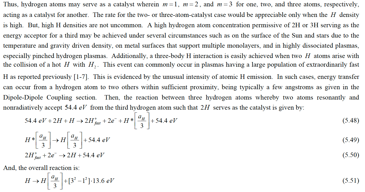
It is interesting to distinguish the magnitude of energy produced in hydrogen combustion and compare it with hydrogen transition state formation with an Ar+ catalyst. Note that each hydrogen atom in the hydrogen combustion process generates approximately 1.4 eV. For the first step in Hydrino formation, transition state formation, (e.g. Eq. 7-5) 27.2 eV are generated, and the second step process will generate as much energy or more. If the proper catalyst is employed (e.g. monomolecular water), BLP estimates the energy generated when a Hydrino is formed will be about 200 times larger per H atom than the energy released by water formation.

Note that the particular process shown in Eq. 7-5 has spectroscopic consequences: electron recapture by Ar2+ means that a 27.2 eV photon should be observed.
There are further rules, as understood by this author, regarding postulated catalysts, or “selection rules” in the language of spectroscopy.
In particular, the energy hole required in Step I of the Hydrino formation process cannot occur between one state in an atom and another, that is to an excited state, in the same atom. Such a process would require the generation of a photon. The RT process does not involve photon addition to the catalyst by postulate.
Thus, the only Type I Hydrino catalysts that are permitted are those in which ionization takes place, and only those ionizations that occur at very nearly an integer multiple of 27.2 eV.
The above requirements are fulfilled by a number of atomic species. Some examples include:
Ar+ → Ar2+, requires 27.62 eV
He+ → He2+, requires 54.6 eV
Monomolecular H2O, which net ionizes with approximately 81.6 eV
There exists a long list of processes that can act as a source of energy holes, but the three listed are most relevant to experimental tests as described in later chapters. A more complete listing of catalytic processes that can accept the required integer multiple of 27.2 eV is found in the first patent issued for postulated Hydrino production processes.4
In terms of observables: the spectra of systems in which Hydrino formation is taking place should have at least one line arising with an energy of m*27.2 eV. This is because the catalytic process creates ions via ionization processes equal to m*27.2 eV (Figure 7-1). These ions will quickly capture an electron, thus returning to their initial pre-transition state production condition, releasing the same energy as required to ionize initially (e.g. Eq. 7-5).
Thus, the theory lends itself to scientific testing to answer several questions:
Are there ~ 27.2 eV photons emitted in Ar/H2 plasmas?
Are there ~ 54.4 eV spectral lines in an He/H2 plasma?
As mentioned above, there are certain molecules that can also act as catalysts. The explanation of the mechanism for these catalytic processes is complex, and involves challenging notation; hence, in this monograph interpretation and discussion is limited to providing a key explanation excerpted from the Source Text. The interested reader is urged to consult the Source Text for further details. To wit:

Type II Catalysts
One catalyst of particular significance to testing of the HH are hydrogen molecules. In this catalytic process two atoms of “fast hydrogen” are created from a hydrogen molecule. Finding the spectroscopic signature (discussed in Ch. 8) of fast hydrogen is one more test of the HH.
In essence the mechanism has two steps:
The hydrogen molecule collides with a hydrogen atom, and;
The product of the collision/reaction are two hydrogen atoms of equal energy, and a hydrogen atom in the transition state.
The two hydrogen atoms, released from the hydrogen molecule, have equal energy, each having one-half that generated by the formation of the transition state. Notably, they must travel in opposite directions in order to conserve momentum.
That is, the energy generated in the creation of the energy hole is converted to kinetic energy. The H atoms imparted with this energy are moving at a not insignificant fraction of the speed of light. They are moving so fast that it causes a Doppler shift of light emitted from excited hydrogen. In the case of easily observed Balmer series lines, this is predicted to lead to broadening of the emission lines which can be observed spectroscopically. As will be detailed in Ch. 8, this H-atom Balmer Series line broadening phenomenon is regularly observed and is of a nature consistent with this proposed catalytic pathway.
The mechanism for this process, generally involving 3 body collisions, is outlined in the Source Text:
This is consistent with the above listed restrictions, an integer multiple of one Hartree of energy absorbed and momentum conservation, are processes that split diatomic molecules, particularly hydrogen. In this type of catalytic process, only diatomic molecules can be catalysts, not single atoms, nor more complex molecules.
These are enormous kinetic energies; hence the H atoms will be moving at spectacular speeds in the laboratory frame, and for this reason the GUTCP predicts Doppler shifts in radiation emitted by excited hydrogen atoms that served as energy holes for the hydrogen to transition state catalytic process. In fact, hydrogen atoms with Doppler shifts in hydrogen Balmer Series lines, consistent with the predictions of the GUTCP, have been repeatedly observed in many laboratories, as well as in stars, as discussed in detail in Chapter 8.
Type III Catalysts
Hydrinos, once formed, can act as catalysts for creation of additional Hydrinos in a process called disproportionation per the Source Text. The catalytic process is, like the other two, a short-range “collision” process requiring physical proximity.
For the most part the disproportionation processes are complex. Herein only a couple of simple disproportionation processes are developed. More detail is available in the Source Text.
A possible disproportionation reaction, resulting in the formation of a much smaller Hydrino is postulated to result from H(1/4) in its stable state (-217.7 eV) absorbing energy sufficient to return it to the transition state at -81.6 eV, that is, 5*27.2 eV (136.1 eV). This energy is created during an energy hole forming collision between an H atom and H(1/4), the net result of which is the conversion of a H atom to an H(1/6) Hydrino.
This process requires the generation of a 136.1 eV energy hole. This is precisely the energy required to promote an H(1/4) Hydrino into its transition state, H*(1/4).
This can be written as:

Where H(1/n) is the nth level Hydrino, and H*(1/n) is the transition state of the nth level Hydrino.
The two processes are energy neutral, and no “signal”/energy is released. Nothing to see here!
One process creates an energy hole (b), and the other process uses the energy released by the energy hole formation to step up in energy (a). As H*(1/n) transition states are not stable, the next steps are immediate transitions to stable states:

There is something to be seen here: two radiative bursts of continuum radiation, Bremsstrahlung type, are anticipated, with total energy of 136.1 eV and 353.5 eV.
Thus, the overall process can be written:

Any process that promotes one H(1/n) to an equivalent H*(1/n) with an integer multiple of m*27.2 eV of input energy, can occur, BUT it must be paired with a second process which generates the needed promotion energy.
Thus, for example, another postulated disproportionation reaction:

Thus, the first reaction (7-10a) requires 27.2 eV, and it is paired with the second reaction (7-10b) that generates that exact energy, and the overall reaction is:

The primary point in these examples: Hydrinos can act as catalysts to create lower and lower Hydrino states. The testable aspect of this postulate is the observation of continuum radiation with specific wavelength cutoffs and energies.
Astrophysics Connection
As discussed in later chapters, there are limited examples of spectra found in Intergalactic Matter that appear to reflect Step II processes.
The conventional astrophysics community has postulated many models to explain EUV spectral lines that are observed. One aspect all have in common: the rather obtuse requirement that intergalactic matter (IGM) is millions of degrees in temperature. This is extraordinarily unlikely in an atomic soup orders of magnitude less dense than Earth’s atmosphere.
Is it possible the published data that indicate IGM is super-hot is based on a misunderstanding of the spectral data? Yes. If the HH is correct, the high energy EUV lines observed emerging from IGM are not indicative of high temperature, but rather indicative of Hydrino formation, probably at very low temperatures. This is discussed in more detail in Chapter 8.
Net outcome: the absence from astrophysical data of the predicted lines arising from the formation of Hydrinos might serve as evidence against GUTCP. The fact that the GUTCP predicted lines are found in this data once again is a failure of experimental data to debunk GUTCP.
Author’s Concerns
The GUTCP Hydrino production model presented in the Source Text contains elements that are of concern to the Author (JP). In brief the primary ones are:
The use of the term “energy hole.”
An absence of explicit consideration of momentum conservation.
The absence of a model of fast hydrogen generation consistent with all data.
The inclusion of a trapped photon in the transition state and final stable Hydrino state.
A simple catalytic path for the formation of some of the smaller Hydrino states.
Each of these concerns is briefly addressed below.
Notably, these “concerns” do not lead to a different set of predicted observables. That is, the observed phenomenon (Chapters 8, 9, and 10) still fail to debunk GUTCP, independent of this author’s quibbles about nuances of the HH.
Regarding the term energy hole- The notion of “negative energy” implicit in the energy hole concept is a bit “metaphysical.” This author suggests for clarity, consistency with standard kinetics, and avoidance of any appearance of metaphysics, to call the process of formation of the transition state a “concerted” reaction.
Regarding conservation of momentum- The conservation of momentum is certainly expected in any classical physics model, including GUTCP. It has significant implications for possible Type I catalysts. As noted above, only species for which ionization requires m*27.2 eV do not create “extra” momentum. This limits the allowed Type I catalysts. It also has Type II catalyst implications. Once momentum conservation is considered, all diatomic molecules, not just H2, appear to be reasonable catalyst candidates, as discussed above.
The third rule of the Step I catalytic process of the HH, one completely consistent with classical physics: allowed catalytic process must not involve a change in linear or angular momentum. This requirement reinforces the restriction of the catalyst to those atoms with an ionization energy very nearly equal to an integer multiple of 27.2 eV. That is, the ionized electron must gain no momentum from the process.
The restriction on momentum conservation means, for example, the energy hole cannot be created such that 75% of a Rydberg of energy is created in the ionization and the other 25% of the required amount is obtained from electron acceleration. Such a process would generate an electron with linear momentum, and this is not permitted by the HH. It would also produce a transition state not at the correct energy state for rapid decay to a Hydrino state.Regarding Fast Hydrogen Generation Mechanism- The data (discussed in Ch. 8) indicates the energy of fast hydrogen is a function of the identity of the Type I catalyst present in the mixed gas plasma (hydrogen + catalytic species). It is clear that the energy of the H atoms follows this trend in Hfast energy as a function of plasma composition: H2/Ar < H2/He < H2O. The current mechanism of line broadening does not suggest this should be true. The proposed mechanism is independent of the composition of the plasma.
Also, the current mechanism requires three body collisions and interpretation of momentum conservation is clearly complicated. It is also clear that more fast hydrogen is found in plasmas containing a Type I catalyst than in pure H2 plasmas or in plasmas containing non-catalytic gases (e.g. Kr) and H2. The proposed mechanism does not explain why this should be the case. The author hopes to see further development of this mechanism. For this manuscript it is simply accepted that Balmer series line broadening is predicted by GUTCP.Regarding the “trapped photon” in the transition state- The trapped photon model implies two types of energy are added to the electron in one step: negative energy (energy hole) and positive energy (photon). Complicated dance. This is one more reason this author does not believe a trapped photon can exist in the transition state. And from where does this trapped photon originate?
The inclusion of a “trapped photon” in the Hydrino- This brings up the issue of stability. Don’t all photons have speed of light components? Any object with components synchronous with the speed of light are in classical physics unstable (Chapter 5). Would not this rule imply “trapped photons” pasted to the Hydrino electron make Hydrinos unstable? There is an explanation provided in the Source Text, arguably too complex mathematically to be entirely persuasive:

Another objection: consistency. To paraphrase K. Popper: an inconsistent theory is not a theory. As discussed in Ch. 6, the excited states of atomic hydrogen consists of a photon pasted to an electron. It is not stable because the pasted photon creates components synchronous with the speed of light.
The decay process for the GUTCP identified unstable atomic hydrogen excited states is simple: a photon is released with energy equal to the difference in energy between initial excited state and the final state. If the final state is still an excited state, per all the transitions from n> or= 3 to n=2, that is, transitions that yield Balmer lines, a trapped photon remains.
Note: this photon is lower in energy than the photon in the original state. In fact, this remaining photon is of an energy that precisely fulfills an energy balance as described in earlier chapters. Moreover, the new photon-containing-excited-state is also not stable (contains components synchronous with the speed of light) and quickly decays to yet a lower energy state by emitting a photon of precise energy required to maintain the final energy balance (See Ch. 8). Again, the energy of the trapped photon in the final state is precisely that energy required to preserve an energy balance. Etc, etc.
Only when the decay leads to a state with no photon is stability achieved, e.g. once the electron in hydrogen decays to the stable, photon-free, ground state.All of the above leads to this point: structurally, the transition state is like an excited state. It is an unstable state consisting of an electron with a photon pasted to it (according to the GUTCP model). So, like the excited state decay process consistency requires knowledge of the energy of the photon in the transition state, and in the final Hydrino state. These values are not available in the Source Text. There is a missing energy balance for the transition state-to-Hydrino process.
And consistency also requires other identical process features. In particular, why isn’t Bremsstrahlung radiation released as an excited state decays? Consistency requires identical structures, e.g., excited states and transition states, decay in the same fashion.
Finally, the notion that a charge-free species, the photon, can impact fields is implausible to this author. It is even more implausible to this author that in some cases a photon decreases the field between an electron and a proton (excited states), and in other cases increases that interaction (Hydrino states). The explanation provided in the Source Text, shown in the excerpt above, is daunting.An alternative photon-free model of transition states and Hydrino states is offered in the next section that overcomes all the above objections, employs simple classic physics, is consistent with all observations, yet predicts the same “signals” as those anticipated by the standard GUTCP theory.
Regarding the simple path to deep Hydrino states- This author has found it difficult to explain how deep (1/n<1/4) Hydrino states form. Perhaps this author is creating a problem that doesn’t exist; it may be the case that deep Hydrino states rarely, if ever, form. Hopefully further experiments will clarify the issue in the future.
For example, Type I catalysts are possible candidates for n=1/2, 1/3, 1/4th states, but are not realistic catalysts for even lower states. Type II catalytic processes to n=1/2, 1/3, and 1/4th have been observed in the laboratory, but not to more tightly bound Hydrino states. Finally, the number of permitted disproportionation reactions is limited.
An alternative pathway to deep Hydrino states is postulated later.

Mod II: An Alternative Photon-Free Model of Transition and Hydrino States
This model below, Mod II, yields the same Hydrino force balance (Eq. 7-3) employed in the Source Text, hence the same Hydrino states found in the Source Text. For this reason it does not change the spectroscopic signals predicted by the HH, and consequently requires no changes in the discussion of experimental (debunking) tests of the Hydrino Hypothesis presented in Chapters 8, 9, and 10. However, the model of Hydrino states presented below does change the description of transition states and Hydrino states. In particular, in Mod II there are no photons in either state; thus, the objections provided in Points 4 and 5 of the Author’s Concerns are overcome.
There are two fundamental changes to the GUTCP model introduced in the Mod II model:
A: The allowed radii are determined on the basis of the postulate that the Rydberg series of energies continues into fractional states (Hydrinos).
B: The hydrogen atom, in all excited states and all Hydrino states, can be modeled as a capacitor with a constant capacitive value.
Regarding A, allowed radii: with the primary postulate of the HH that Rydberg states continue to fractional values, the radii of these states can be computed without employing an energy balance. That is, instead of employing a force balance, simply solve for radii using equations introduced in Ch. 4:

where, per traditional orbital mechanics, the binding energy (EB) is equal to the kinetic energy. And note, to solve for the radius rather than the velocity, the conservation of angular momentum equation, mvr=h-bar, is employed, as in Ch. 4. In short, this equation is solved:

Where EB must be one of the allowed Rydberg energies, values found in the right most column of Table 7-1. Using the values for constants found in Ch. 4’s Table 4-1, and noting that energy must be expressed in Joules (1eV=1.602177e-19 J), the allowed radii, r*, are readily found to be the same values listed in Table 7-1: aH/2, aH/3, aH/4 etc. Notably, there is nothing non-GUTCP regarding the determination of allowed radii.
B: It is postulated that the hydrogen atom has a constant capacitance, and from this postulate a functional form of the dielectric constant is derived. That is, the hydrogen atom, in the excited states, ground state or Hydrino state, can hold exactly one unit of electron charge. Definition of capacitance:

Where C is the capacitance, Q is the charge, V is the voltage and e is the dielectric constant (an italicized e will denote the term epsilon). In Mod II it is accepted that C and Q are constant for the ground state and all excited and Hydrino states.
Is the voltage constant for all the listed states? No, but e*V can be effectively constant if e is allowed to change in a regular fashion. This formulation allows capacitance, (Eq. 7-13) to be constant. Thus, the objective now is to find a simple expression for e in terms of radius.
Voltage for an orbitsphere surrounding a nearly “point” nucleus can be determined from this standard classical physics equation:

Where Vr0 is the voltage of an orbitsphere of radius r0. It is also assumed that the nucleus is essentially a point particle, a good approximation relative to the orbitsphere.
This equation is easily solvable when we use the proper expression for the field of a point charge. Classic physics indicates the field of a point charge in classical physics decreases as (distance)-2, per this equation:

Where e0 is the permittivity of free space. It should also be noted that there is no field inside a superconductor, a class that includes orbitspheres, as discussed in Ch. 5. Thus, the only field that arises as the orbitsphere shrinks from an infinite radius to its final radius r0 is that of the proton, assuming a charge of unity. Thus:

The takeaway from Eq. 7-16 is that if the voltage is decreasing proportional to 1/r, then to make the capacitance of a hydrogen atom constant (Eq. 7-13), the value of e must be proportional to r. Moreover, e must be dimensionless for the units of Eq. 7-1 to be correct. Note: Similar analyses are found on the web (Figure 7-3).
Thus, the equation for capacitance becomes:


Figure 7-3: Independent Development of Formula of Capacitance For Concentric Spheres. Note, the derived equation is identical to that when the inner sphere diameter, a approaches zero, the equation for capacitance above is the same as Eq. 7-17. It is assumed in the GUTCP hydrogen model that the nuclear radius is << than the orbitsphere, thus, a~0.
Also, it is necessary that the final force balance “collapse” to that of Eq. 4-5 when r=aH:

In sum, for atomic hydrogen capacitance to be constant, and the force balance equations to yield the correct values when r=aH , and for the e to be dimensionless, the correct functional form for e as a function of the radius of the hydrogen atom is:

Where r*, as explained above, are the allowed radii per the assumption of the Rydberg series energies, r*=aH/ 2, aH/3, etc…

We deploy the functional form of e to properly correct force balances for the case that e is not equal to e0, both for the excited states and for the Hydrino states. The force balance developed, based on hydrogen having constant capacitance, an equation that replaces both Eq. 6-1 (excited states) and Eq. 7-3 (Hydrino states) follows:

There are only specific values for r*, hence n, as explained above, and in Chapter 6. For Hydrino states, n is fractional, n=1/2, 1/3, 1/4…1/137. For excited states n is a natural number, per Table 6-1, n=2, 3, 4…
Some may object to Mod II on the basis that it requires a functional form for e, rather than a constant value. In reality the dielectric constant for macroscopic systems, e, is different for each material, and for each material it is a function of field strength (Figure 7-4), temperature, frequency, and other parameters. But isn’t the inside of an atom “free space?” Isn’t virtually all the space in any material, which is composed of atoms, “free space?”
Yet, in real materials the dielectric constant varies from ~1 (air) to 1010 (Refs. 7-6, 7-7). Hence, it is reasonable to postulate, per Mod II, that the space inside an orbitsphere is not free space, and hence the permittivity of free space cannot be used for the “inside” of an orbitsphere without dielectric correction.
Another reasonable objection: how is the value of e related to the force experienced by the orbitsphere? Clearly, Eq. 7-1, Mod II indicates there is an inverse relationship between e and the force experienced by the orbitsphere. Is this correct? That is, does a smaller value of e lead to a greater force operating on the orbitsphere?
In brief: Yes.
Let us consider the parallel plate capacitor for the purpose of providing a fundamental, but qualitative, rule of the relationship between force and e. Start with this well-established general rule (Refs. 7-6, 7-7): the larger the value of e, the better the dielectric is at cancelling the field created by the charges on the plate. That is, the larger the value of the dielectric constant of the material between the electrodes, the smaller the field at every point in space, including at the electrodes.
Imagine an experiment in which the force on two flat electrode plates, of constant separation and constant charge, is measured as a function of the dielectric placed between them. As the dielectric constant of the material placed between the plates increases, the force on the plates is found to decrease. Why? As the dielectric value of the materials tested increases, each plate “sees” fewer net charges, hence “feels” less force, due to field cancellation which “improves” as the dielectric value increases. Put another way: the higher the dielectric value of the tested material in the Gedanken experiment, the smaller the field at the plates.
This is summarized as General Rule Dielectrics One (GRDO): as force on the plates is proportional to the electric field, the higher the value of e, the lower the force pulling the constant distance, constant charge, electrodes together.
In the case of the force balance on an orbitsphere (rather than a parallel plate electrode), consider the fractional states. As the value of the “fraction” gets smaller, the value of e also decreases, thus the stronger the anticipated force on the orbitsphere. That is, the “empty space” between the proton and the orbitsphere loses progressively more ability to cancel field as that space gets physically smaller. GRDO, per Eq. 7-18, is honored. It is also clear the rule is honored for excited states as well.
There is also data consistent with e decreasing as the field between the electrodes of a parallel plate capacitor is increased. This is due to saturation of the dielectric material (Fig. 7-4) as shown in Figure 7-5. It is argued, this experimental result is analogous to that observed with the orbitsphere. As the orbitsphere size decreases, the field increases, as in Figure 7-5, and the value of the dielectric will decrease.

Figure 7-4: Typical Ceramic Dielectric Polarization Curve. The dielectric constant is proportional to the slope of the polarization curve. Clearly the dielectric constant is not constant. From ~-10 to +10 volts it is nearly constant, but at higher absolute voltages the slope and hence the dielectric constant sharply decrease, due to saturation, full alignment, and maximum magnitude of the dipoles in the dielectric. Theory developed elsewhere.56
Consider the issue of stable Hydrino states from a fresh perspective, a sort of “Mod II backwards” approach: should the (near physics folklore) notion of the continuation of the Rydberg energies to fractional states be a guide to theory, or a natural outcome of the application of the fundamental laws of physics? Could there be “Hidden Variables” leading to the Rydberg series energies? Is it possible that combining the requirements of force balance, momentum conservation, and constant capacitance, per Mod II, lead naturally to the Rydberg series energies? Certainly, all three are consistent with equations established prior to 1871 per the original requirements of the GUTCP. Advantages also include no need to modify the classic Coulombic interaction force, and consistence with the stability criteria.

Figure 7-5: Capacitance and Dielectric Values Decline in Saturated Region. As the applied voltage increases, all dipoles gradually align with the applied field in the Normal Field region ( < ~|20 kV/cm.|) At this point full saturation is achieved and the dielectric is not capable of further “field cancelling.” This result in a near linear decline in the measured capacitance (TOP) and dielectric (“Relative Permittivity”) value (BOTTOM) with further increases in the applied field (Saturation Region). (After Ref 7-7).7
In sum, Mod II yields one force balance equation that works for all forms of hydrogen: excited states, ground state (n=1), and Hydrino states.
This single equation is identical to the GUTCP force balance for both excited and Hydrino states, hence yields the same energy levels, radii, etc. This means both the GUTCP model and Mod II predict the same signals. Experimentally, the argument is butter on top of the bread versus on the bottom (Figure 7-6). Nada difference.

Figure 7-6: Butter Battles. From Dr. Suess, ‘The Butter Battle Book,’ Random House (1984).
So, why develop or consider Mod II? The following are the reasons:
Mod II is more self-consistent than the GUTCP version in several ways:
A: The transition state in Mod II does not have a photon, hence it is different than a photon containing excited hydrogen state. States without photons (transition states) cannot lose energy via photon loss. In fact, based on decades of experimental results, Bremsstrahlung is the anticipated energy loss mechanism for “naked” electrons.
In sum: in the GUTCP model both transition states and excited states consist of an orbitsphere with a photon pasted to it. Thus, transition states and excited state should lose energy in the same fashion. However, the GUTCP stipulates transition states and excited states lose energy in completely different fashions as the electron falls to a lower level state. Not consistent. Contrast: In Mod II, excited states and transition states are different (photon vs. no photon) hence should collapse to lower energy levels via distinctly different mechanisms, as observed (Chapter 8). Consistent.
B: In the GUTCP it is postulated that, based on classical physics analysis, states with photons attached are unstable. Yet, it is also postulated that Hydrino states both have photons and are stable. Inconsistent. In contrast, Mod II Hydrino states do not contain a photon, and in terms of classical physics are expected to be stable, as observed. Consistent.
C: The GUTCP-predicted release of energy via Bremsstrahlung in transition from transition states to Hydrino states is not consistent with excited states, with the same structure as transition states in the GUTCP, not releasing Bremsstrahlung radiation during jumps to a stable lower energy state. Experimental results clearly show no Bremsstrahlung as excited states lose energy.Other issues overcome by Mod II:
A. In Mod II, there is no need to puzzle over how in the formation of a transition state an energy hole is absorbed, AND simultaneously a photon produced. There is no photon.B. In Mod II there is no need to puzzle over the magnitude of energy of the photon in either the transition or Hydrino state. There is no photon.
C. In Mod II there is no need to puzzle over the suggestion that trapped electromagnetic energy (photon), containing no charge, can influence field strength. There is no photon.
D. In Mod II there is no need to puzzle over how the “polarity” of a photon can determine whether a photon blocks field (excited state), or enhances it (Hydrino state). There is no photon.
E. No need to puzzle over how the photon “knows” the value of the quantum number n, and adjusts its blocking/enhancing power accordingly. In Mod II, the value of n in the force balance can be traced directly to two postulates: i) the postulate that the only stable Hydrino states are those with Rydberg series energies, and; ii) the constant capacitance postulate.
All the physics in Mod II are pre-1871. Indeed, M. Faraday originated the concept of dielectric and different materials having different dielectrics (or different dielectric constants). Suggesting photons can block or enhance fields is definitely not pre-1871, not classical physics, hence somewhat outside the requirement of GUTCP that only classical physics is invoked.
Final argument for Mod II: Occam’s Razor.
A Proposed Mechanism for Forming Deep (n>4) Hydrino States:
Perhaps there is room to advance another path to deep Hydrino (n>4) states: a transition state can directly transition to any Hydrino state. There may be preferred transitions, but transitions to any Hydrino state are allowed.
This idea is not described in the GUTCP. As we saw above, in the GUTCP model, there exists a linear relationship between the amount of the energy transfer to the catalyst species and the final Hydrino state formed. However, there is no classical physics objection to this postulate by this author, and there is a type of precedent.
Precedent: the Balmer series describes excited (“transition state?”) hydrogen states moving to the n=2 final state and the Lyman series arises from excited hydrogen electrons moving to the n=1 state. Clearly, the identity of the initial state does not determine the identity of the final state. There is no energy law, no momentum conservation issue, etc. with this postulate. The allowed transitions which could produce light in the EUV range, are listed in Table 7-2.
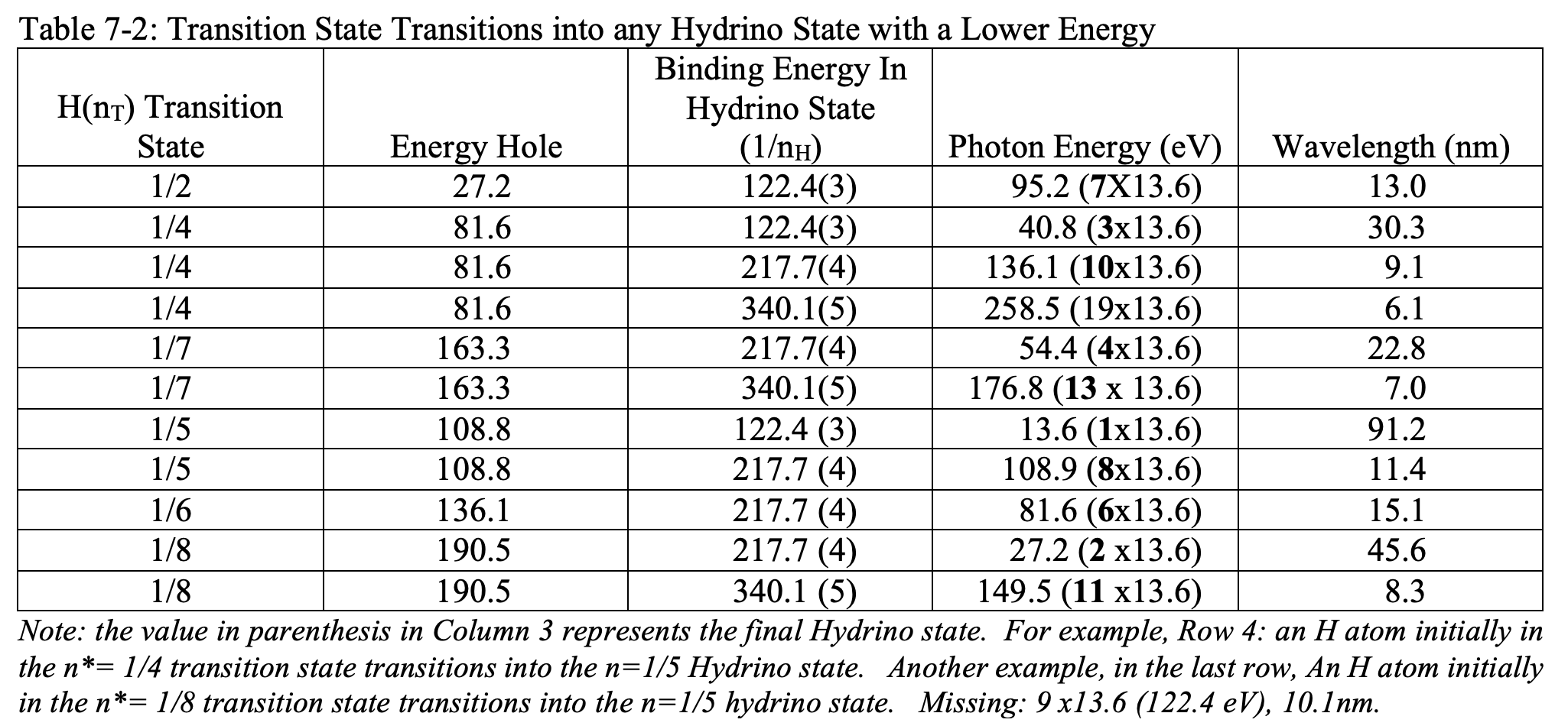
It is notable that between them Tables 7-1 and 7-2 predict processes able to produce low edge energies that are multiples of 13.6 eV, that is potential energy of release are 13.6 x 2, 3, 4, 5, 6, 7, 8, 10, 11, and higher. It appears only 9 x 13.6 = 122.4 eV is missing.
It is also notable that this mechanism is less “hindered” in Mod II than in the GUTCP model. In the GUTCP model properties required of the trapped photon in the transition and Hydrino states may prohibit this mechanism. Unclear.
In sum, this postulate helps explain the formation of deep Hydrino states, and experimental observation consistent with the formation of such states (Ch. 8).
Hydrino Formation Observables
At this juncture it is valuable to review the GUTCP-predicted forms of radiation that should be observable.
From Step I:
One: radiation arising from recapture of free electrons, created in the energy hole generation/absorption process by ionized catalyst species. These processes should create normal, narrow, spectroscopic lines with wavelengths corresponding to m*27.2 eV.
Or -
Two: atomic hydrogen Balmer series line broadening from super-high kinetic energy hydrogen generated from processes in which hydrogen molecules act as catalysts for generation of transition states.
From Step II:
Three: Bremsstrahlung-type radiation, that is, broad spectral bands as transition state hydrogen falls into a final stable Hydrino state. These bands will have very specific maximum energy corresponding to the energies listed in Table 7.2 and 7.3. The energy release may also come in the form of third-body kinetic energy.
Experimental testing designed observe the above listed observables is presented in Ch. 8.
Personal Notes
Note 1: Existence of Cosmic Karma
If there is some truth to Mod II would that demonstrate Cosmic Karma? Why would I have studied both GUTCP and capacitors for decades if that were not the case?
Note II: Classical Basis of the Uncertainty Principle and Implications for Photons
Summary: there is a classical explanation for the quantum Uncertainty Principle. This classical explanation inspires a new notion of the nature of photons.
Classical Uncertainty
Classical basis for the Uncertainty Principle: one of my earliest conversations with Randy regarded the issue of line widths for emitted photons and gamma rays. As this occurred decades ago (~ 1996), the best I can do at this time is present a “best recollection;” however, I think the essential elements of this report of the conversation are accurate. And the very interesting conclusion reached: there is a classical explanation for the quantum Uncertainty Principle, is also accurate.
The topic of the conversation was a challenge to Randy and the GUTCP (or whatever it was called at the time): based entirely on classical laws, explain all spectroscopic observations as accurately as standard quantum theory (SQM).
Randy wanted a specific example, so I brought up the Uncertainty Principle and its application to the observation of different line widths for different photon emissions.
Note: line width in spectroscopy is the full width, at half-max height (FWHM) of the generally Gaussian diffraction peak observed for a peak associated with a photon at a given energy and wavelength (Figure 1). The experimental fact is, possibly contrary to intuition, the “lines” observed in spectroscopy are never simply a single line at a single wavelength. The observed lines, often Gaussian-shaped peaks, always span a range of frequencies. The shapes differ for different processes.

Figure 1: Schematic of Observed Spectroscopic “Lines.” The shape of the spectroscopically observed diffraction lines are characterized by the Full Width at Half Maximum (FWHM). Different processes produce different FWHM.
I noted in our discussion that SQM could explain the origin of variable line widths using the Uncertainty Principle. In the applicable variant of that principle: it is not possible to know both the exact energy, and the exact lifetime of a particle.

For an electron in an atom, or molecule, transitioning from an excited state to a stable ground state, this means there is uncertainty in the energy change of the process. There is no “exact” energy of transition. There is always some lifetime (Dt) of the excited state, hence some uncertainty in the energy (DE, proportional to FWHM, Fig. 1) of the event. This uncertainty is reflected in uncertainty in the energy of the photon emitted as an energy conservation outcome of the process.
The value of Dt is the lifetime of the electron excited state; hence the uncertainty in the energy of the transition, and also the emitted photon energy is:

In practice, this uncertainty in the photon energy has spectroscopic consequences. As line width for a spectroscopically measured photon, in wavelength, is proportional to DE, the shorter the lifetime of the excited state, the wider the line width of the emitted photon in wavelength. For example, in Figure 1, the greater width of the plasma absorption line suggests plasma absorption is a shorter time process than the reference process. In terms of photon emission when an excited state decays to a ground state, a long-lived excited state (Dt large) leads to less uncertainty in emitted photon energy, and consequently a narrow emission peak in k-space.
Randy quickly explained that this “quantum uncertainty” is actually a classical physics result. He noted there is no need for quantum to explain the line broadening phenomenon at all. There is, and always has been, a classical physics Uncertainty Principle!
To wit: imagine a long string under tension. Give it a very quick pinch at one end, and a “wavelet” travels toward the other end at a relatively slow speed, certainly compared to the speed of light (Fig 2).
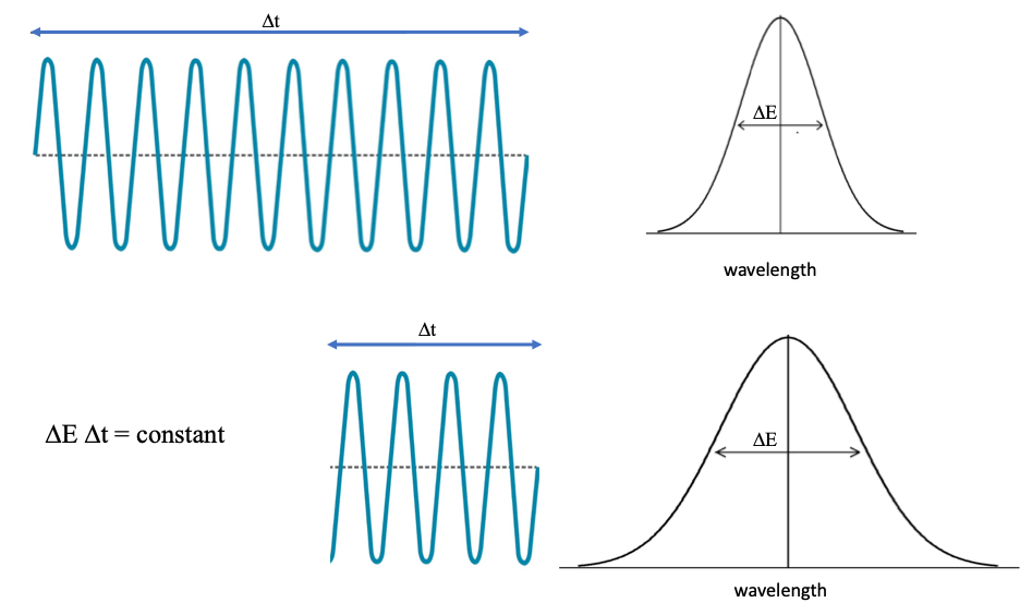
Figure 2: Wavelets on a String. The length of the wavelet traveling on a string is a function of how long the “pinch” took. A longer pinch (TOP Left) yields a physically longer wavelet length relative to a short pinch (BOTTOM left). The peak width in k-space (DE) is inverse; the shorter wavelet produces a broader k-space peak than the longer wavelet, per the “Classical Physics Uncertainty Principle,” DE*Dt = a constant.
In classical physics the wavelet cannot be described as having a single frequency, but rather is described mathematically as having a number of frequencies of significant magnitude. The mathematical description in wavelength space will likely be a Gaussian peak (Figure 2, right side), just like the shape of a spectroscopic “line” from an event creating a photon (Figure 1).
In wavelength space (k-space) the traveling wavelet on the string is described as a wave packet. Indeed, in classical physics only an absolutely flawless wave of infinite length can be described with a single frequency. Typically for a short duration/length wave in any media, the following relationship, herein labelled the “Classical Physics Uncertainty Principle,” holds:

Thus, if the string is pinched for a longer time, creating a longer wave packet, the uncertainty in DE is reduced, and vice versa (Figure 2).
Now, note the similarity of Eqs. 1 and 3. Assume for photon producing atomic processes, the value of the constant in Eq. 3 is h-bar, this makes Eq. 3 the same as Eq. 1! That is, both classical physics and quantum physics predict the same uncertainty relationships!
Thus, Randy concluded, the classical physics description of a wave on a string, can be used to predict the “uncertainty” of spectroscopic lines. There is no need for a “Quantum” Uncertainty Principle to explain spectroscopic line widths!
Photons
First note: none of the above dialogue is reflected in any element of the Source Text. In the Source Text the photon emitted from an atom transitioning from an excited state to an SQM “ground state” is a particle of definite shape. Indeed, it is approximately the same size and shape as the electron in the excited state to which it was “pasted.”
It is also important to note that Randy’s explanation of a classical uncertainty principle is the inspiration for the model below.
Now, allow some apostate thinking: that is, deviate both from SQM and the GUTCP. Specifically, consider this proposed model of a photon: a photon is a wavelet of wave shaped radiation (Figure 2, left) of finite size. Positive aspects of this model:
It is an object in 3D space, as required of all particles in the GUTCP.
A wavelet of finite size could (?) exhibit properties of both waves (diffraction) and particles (photoelectric effect). Possibly this is a simpler means of explaining how a photon can be responsible both for the photoelectric effect (particle behavior), and diffraction (wave behavior). In this author’s mind, both the GUTCP and standard paradigm physics do not smoothly explain how their photon model explains both known experimental observations. And does this proposed model also work as an explanation for Compton scattering?
A photon becomes just another form of E and M radiation, not something remarkable and unique. That is, all forms of radiation, photons, microwaves, radio waves, EUV radiation, and Bremsstrahlung are all “wavelets.” Also, these wavelets could have a number of shapes, as long as they are of finite extent in space-time: i) Spherical, like waves going outward from a rock dropped in a pond (except 3D), ii) directed, like wake created by a boat plowing rapidly through calm water (except 3D), iii) cylinders, etc.
The model suggests an explanation of phenomenon such as excited state lifetimes. For example, it takes time to “unwind” a spherical trapped electromagnetic bit of energy in an orbitsphere and transform it into a photon-wavelet, traveling at the speed of light, of specific length.
Consider Point 3. Figure 3 suggests how wavelets of various shapes, containing multiple frequencies, and non-constant magnitudes, will be observed in k-space.

Figure 3: Postulate: All Forms of Radiation are Wavelets. Even irregular and short pulses of radiation (BOTTOM) can be transformed into k-space (TOP) “lines” or peaks. If multiple pulses are generated by a macro process (e.g. slamming super high energy electrons into a wall), a non-Gaussian wave form (TOP) will be recorded by a spectrometer. In this model, not only photons are diffracted, but “wavelets” of many shapes of radiation, from many sources.
Example Point 4: Let us consider the lifetime of excited states. In particular, the lifetime of an excited hydrogen atom, generally reported to be about 10-8 seconds, reflects the time required to produce a wavelet from the trapped electromagnetic energy in the spherical chamber of the orbitsphere. This raises the question: how long, in 3D space, is a wavelet that requires 10-8 seconds to be fully generated? Given that the speed of light is approximately 3*108 m/sec, the wavelet would be about 3 meters long:

This is clearly only a ballpark figure. The process of unwinding may involve multiple steps such that only a fraction of the observed lifetime, Dt, is reflected in the actual generation of the wavelet. In that case the wavelet would be shorter than the 3m computed above…
The above is merely a thought experiment. There are undoubtedly many difficulties with the model. For example, the model requires some work to make it consistent with the concept introduced earlier that a photon travels on the infinite field of the electron from which it originated, and not in some universal space. Also, if both a rapid and a long process release the same energy, how is the energy accommodated in the photon? Lots of possible answers exist. For example, assuming the particle-photon introduced here has a cylindrical shape, perhaps the diameter reflects energy conservation. Perhaps a long photon would have a smaller diameter than a short photon. Is energy proportional to total photon volume? And then there are clear questions about dynamics. How is such a macro particle trapped by an orbitsphere?
Final thought: are there physical analogies to photons converted into instant energy, that is some macroscopic physical process analogous to near instant “quantum level” conversion of wave energy to particle energy, such as the photo-electric effect? Postulate: the energy of a “wavelet” traveling on a whip converted instantly into sonic boom energy is an example of a traveling wave “instantly” converted to physical energy in macroscopic classical physics.8 The very rapid conversion of mechanical wave energy to an energy pulse/shock wave is a macroscopic process somewhat analogous to the photoelectric effect in which the energy of a wave-particle photon is “instantly” transferred to increasing the energy of a particle (GUTCP electron).
Just thinking out loud, a process enabled by the GUTCP, but forbidden by the physics cancel culture guardians, that is, those who protect the Physics Community democracy rules:
Rule #1: Everyone gets to vote on the best theory.
Rule #2: There is only one theory allowed on the ballot…
Note III: The Scientific Brotherhood of Hydrino Dreamers
One of the most rewarding aspects of participating in the Scientifically UNwoke exploration of alternative quantum paradigms are the people I’ve met who made the same choice: to be open supporters/gamblers for a contrarian cause.
Having a stake in an enterprise such as BLP has been remarkable fun. We shareholders are effectively an informal brotherhood of gold seekers. Everyone attached to the project is looking to get rich and/or gain some psychic gold.
There is more than a passing resemblance between our physics brotherhood and the brotherhood of folks attached to “The Curse of Oak Island,” my favorite reality TV show (note: this is not an affection I have previously publicly embraced). Indeed, in both cases only the willingly optimistic can see a positive outcome, an actual identifiable prize, being rewarded in anything but a very hazy future. And yet, everyone involved has a positive outlook and a conviction that success will arrive.
The largest group of contrarian clubbers are those who claim be interested in the GUTCP as a path to fantastic riches. A standing topic is the size of the yacht each will buy. Clearly, this is a slow path to riches because many in this group invested one or even two DECADES ago and are still waiting for the (hopefully) inevitable commercial application of Hydrino technology.
I hold a special spot in this particular brotherhood as a “sub-guru.” Clearly, I’m not Randy. Indeed, I’ve struggled for years to understand just a small fraction of GUTCP. The scope of his genius is nearly unfathomable. Still, I do possess enough training and wit to fully understand at least part of the most relevant technical aspects of GUTCP. And I’ve developed a narrative to explain it to those with patience to listen.
My credentials: in some of the early versions of the GUTCP book there is a picture of all the staff of what was then Black Light Power (before the name change to Brilliant Light Power), with me standing in the middle just to the right of Randy. I’m proud of that picture, and I like to think for a time I was the Right Hand Man. And, I am a co-inventor on the first BLP patent and have co-authored six papers with Randy.
For a few years I even served as an emissary for BLP, giving talks for BLP (Italy, Houston, etc.) that might lead to investments or collaborations.
I have several roles as the Gold Club sub-guru. First, I am sometimes asked by its informal members for reassurance that the fundamentals of Hydrino formation as written by Randy make sense and are consistent with observation. I have consistently provided reassurance: the standard paradigm of SQM is clearly nothing but mathematical gibberish and physical fantasy, whereas the GUTCP makes physical sense, contains no new physical laws, and its prediction are quantitatively very close, with no adjustable parameters, to all observations.
It is EXCEPTIONAL science.
I have also explained why, generally, the scientific establishment despises the theory: no one likes a party pooper…and the quantum folks have been partying and spending other people’s money in great quantities for many decades.
Second, I have been asked for estimates of the timeline to a BLP prototype. This is a kind of engineering question. For this I have some credentials. I was a Prof. of Chemical Engineering for nearly two decades, so I do have a general sense of engineering timelines. I have also worked on industrial projects.
For example, I worked under contract on a next generation battery anode design for Toyota for three years. I learned from my Toyota contacts that the Prius was born on a gamble. The company made a conscious decision to make a hybrid vehicle and were prepared for a long-term investment, on the order of 10 years, from idea to commercial vehicle.
The biggest hurdle was inventing a battery that had the power density and stability to operate without fail for several hundred thousand miles. Thus, the ten years included a couple of years doing laboratory work on several potential novel battery anodes and cathodes, followed by a down select and another year of battery building and lab scale testing.
Next, the final battery had to be designed and built, followed by building a production line: another couple of years and a LOT more money. This was followed by installing the battery in a test vehicle and running it on a track for a long time. The battery design and the factory were iteratively improved, guided by test results. Finally, a factory was built for the car that would house the battery, followed by more testing, and more improvement. Rome wasn’t built in a day, nor was the Prius.
I also learned that the modern capitalist economy is built by gamblers. Clearly, Toyota was gambling. They didn’t know for certain the battery or car would be an engineering success. They didn’t know if it would be economical to build. And they did not know it would have an audience. They won all the bets, and my Toyota contacts told me for a time the company thought of itself as a battery company, not a car company, because it was the battery that made them unique in the marketplace. The Prius and the new battery made Toyota one of the largest car companies in the world. Just to be clear, I was not involved with the Prius. I had a small project for the next generation battery: designing, building, testing, analyzing a novel Sn/C battery anode. Long story about a new gamble.
Clearly all those involved in the BLP enterprise, including all members of the Gold club, are gamblers as well.
Finally, Randy is a gambler. He once told me that if money was his only objective, he would have cashed in on his Harvard medical degree and done very well economically. Instead, he started a long-road gamble, the first five years of which were spent as a laboratory assistant at a small college, while living over a Wendy’s.
Is gambling an essential ingredient in our modern economy?
So, what timeline prediction did I make for curious Gold Club members, based on my experiences, for a BLP commercial product?
Given my experience with several companies steeped in development of new technology, with a realistic approach to the problem, I concluded it takes at least SEVEN years for a new product based on an actual, and novel, physical thing to become commercial. A product based on information technology, not a physical thing, appears to take about half as long.
Anyway, five years ago, I took all the information I had about BLP and the SunCell, my general understanding about the timeline to engineer a product, the advantages to having a super-genius in charge of an engineering project, etc. put all of it in my mental mixer, and announced this conclusion: do NOT expect a commercial product in the form of a Sun Cell any sooner than the summer of 2024.
I hope the Suncell is commercialized, or I am going to have to explain myself to some unhappy fellow travelers, and I will lose a bet to one of my best friends, a physicist/astronaut who is not a Gold Club member. Look, I’m gambling, something most scientist eschew!
I’ve also had extended relationships with others in the BLP orbit, including others writing about BLP. During the research phase of this monograph, I’ve had multiple extended calls from the authors. It’s fun, and interesting to follow the outcome. In one case I was featured in an entire chapter, in the other in an entire sentence. And, I was gifted the original of one of the figures from one of the books. It holds a prominent place on a bookshelf in my home.
There are also BLP “watchers.” Many folks involved in other “alternative” energy, particularly those in the Low Energy Nuclear Reactions (LENR) space, are watching from the sidelines. Once it is understood I am from the GUTCP side of the tracks different reactions ensue.
Some, like my friend Ed Storms, are open to the notion that the GUTCP and Hydrino formation may explain much of the results associated with excess heat in LENR experiments. This author believes that it is not a coincidence that most LENR experiments bear a striking resemblance to Randy’s early Hydrino reactors. Others among the LENR enthusiasts have ranted at me publicly for daring to challenge SQM. “It is the most beautiful and sublime theory in history!” one ranted, “How dare you question it!” But most are more circumspect, and very curious.
I interacted for years (until about 2006) with the business leaders of BLP for purposes of organizing contracts, making visits to present an independent assessment, and I believe I have been very independent in my communications to interested parties/potential BLP supporters, etc.
Apropos of these interactions is a recent encounter. I was trying to raise money for a small company I started, Capacitor Foundry, and found myself speaking to an old friend from college, who it transpired was a 50/50 partner in a multi-billion-dollar energy project with one of the former business development folks I worked with at BLP before he was exiled, like me. Small world.
Once, while visiting a major oil company research headquarters for the purpose of giving a talk for a group of engineers and scientists there regarding BLP and the GUTCP theory, a team formed by the company to critique and select for funding paradigm shifting technologies, I asked if I could see an old friend from graduate school. I only knew he worked for this oil company as, except for annual Christmas cards, we had lost contact.
In grad school he sat in the office next to mine, and played shortstop on our intramural softball team while I played second base. We were great friends. My corporate host looked at me oddly after my request and said nothing. My friend did show up for the presentation, and the talk went well. I was prepared to end it after an hour, but the audience, fascinated, asked me to continue. The presentation continued for over two hours! Only afterwards did I learn my friend was THE Chief Engineer for the company world-wide. Small world. Sorry, no investment in BLP followed.
Our unofficial club is modern in the sense that we rarely meet, but less than uber-modern as most of our conversations are over the phone, albeit the cell phone. Not Zoom. But occasional and unstructured interaction are not conducive to the exchange of excellent ideas or forming science and engineering collaborations. We need a new format.
One model I admire: historic science societies where all members were in a small geographic area, electronic communication did not exist, hence it was essentially mandatory for members met in the flesh on a regular basis. That model clearly led to some fantastic science!
Royal Society of London is a prime example:

So, in conclusion, I don’t want a yacht, but it would be great to have enough funding to start something as marvelous as the Royal Society of London, but perhaps we could find a snappier name like, “Hydrino Yacht Club.”
Membership will not be limited to those with science credentials. This treatise clearly shows some of the best science is not done by credentialed scientists. Indeed, in the case of the GUTCP, the mores and strictures of traditional academia has profoundly hindered advancement and testing of a superior theory. We need a new model, separate and apart from the moribund status quo.
Our society will be open to all with open minds, not wedded to any narrative, possessing an understanding of the scientific process. Entry will require passing a test regarding the true nature of the scientific process and some basic philosophical knowledge of epistemology, as well as the demonstrated ability to distinguish propaganda from evidence-based conclusions. Very small group.
And possibly, we will meet on BLP Gold Club member’s yachts…
A.I. Arbab, “The Fractional Hydrogen Atom: A Paradigm for Astrophysical Phenomena,” Journal of Modern Physics 3(11), 1737–1743 (2012).
D.C. Tsui, H.L. Stormer, and A.C. Gossard, “Two-Dimensional Magnetotransport in the Extreme Quantum Limit,” Phys. Rev. Lett. 48(22), 1559–1562 (1982).
N. Laskin, “Fractional quantum mechanics,” Phys. Rev. E 62(3), 3135–3145 (2000).
R.L. Mills, W.R. Good, J. Phillips and A.I. Popov, “Lower Energy Hydrogen Methods and Structures,” US Patent 6,024,935 (2000).
J. Phillips, “Theoretical and experimental basis for the super dielectric model of dielectric materials,” Physics Essays 33(3), 306–318 (2020).
F.J.Q. Cortes, A. Suarez, and J. Phillips, “Towards a Universal Model of High Energy Density Capacitors,” in Innovations in Engineered Porous Materials for Energy Generation and Storage Applications, (CRC Press, 2018).
G.J. Reynolds, M. Kratzer, M. Dubs, H. Felzer, and R. Mamazza, “Electrical Properties of Thin-Film Capacitors Fabricated Using High Temperature Sputtered Modified Barium Titanate,” Materials 5(4), 644–660 (2012).
A. Goriely, and T. McMillen, “Shape of a Cracking Whip,” Phys. Rev. Lett. 88(24), 244301 (2002).
Dr. Mills has the only sensible solution to the sub-atomic world!
It is brilliant and internally consistent.
What s needed NOW is just ONE “Over Unity” and “Reproducible* device and the Entire World will change!
Thank you for this excellent introduction to the hydrino form of hydrogen!
The word "hydrino" seems to be substituted in error for the correct word "hydrogen" in the first sentence of the second paragraph under the subheading "Step 1 of Hydrino Formation".
In the first step of the process, it is atomic Hydrogen (not Hydrino), which transfers m*27.2 eV to a catalyst species that can accept that amount of energy.
Correcting this small error will be helpful to the understanding of newcomers to these concepts.
Of course, in subsequent steps, Hydrino itself can become a substrate reagent in a hydrino reaction which takes, for example, 1/2-radius Hydrino to a smaller fractional electron orbitsphere number of Hydrino.